Super-resolution with SRResNet

Single-image super-resolution (SISR) is the inverse problem of recovering a high-resolution (HR) image \(x\) from a low-resolution (LR) observation \(y = \downarrow_s(x)\), where \(\downarrow_s\) denotes downsampling by factor \(s\).

Unlike physics-aware methods in DeepInverse (iterative algorithms, unrolled networks, diffusion models) that require the forward operator at inference, SRResNet [1] is a direct feed-forward network: it maps LR images to HR estimates in a single forward pass without needing the degradation model at test time. Inference is simply model(y).

This example demonstrates:

1. Inference with weights pretrained on DIV2K for 4× RGB bicubic super-resolution.

2. Fine-tuning with deepinv.Trainer to show the model is fully trainable.

import torch
import matplotlib.pyplot as plt

import deepinv as dinv

device = dinv.utils.get_device()

Selected GPU 0 with 21592.4375 MiB free memory

1. Inference with pretrained weights

The default SRResNet was trained for RGB 4× super-resolution on DIV2K under the L1 loss, using DownsamplingMatlab (MATLAB-style bicubic downsampling, factor 4), ADAM with lr 5e-4 at batch size 16, and random 128×128 HR crops for 400 epochs.

Note

The pretrained checkpoint uses the default architecture with final_relu=True.

model = dinv.models.SRResNet(pretrained="download", final_relu=True).to(device)

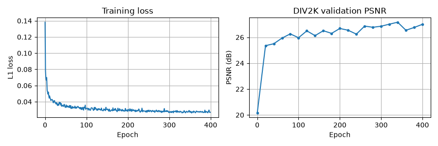
We can visualise the training loss and validation PSNR on DIV2K stored inside the checkpoint.

Note

The validation PSNR in the checkpoint was computed on the luminance (Y) channel only, as is standard practice in SISR benchmarking. The PSNR values shown later in this example are computed on all RGB channels and will therefore differ.

ckpt = torch.hub.load_state_dict_from_url(
    "https://huggingface.co/deepinv/srresnet/resolve/main/srresnet_ckpt.pth.tar",
    file_name="srresnet_ckpt.pth.tar",
    map_location=device,
    weights_only=False,
)

loss_curve = ckpt["loss"]["SupLoss"]
psnr_curve = ckpt["eval_metrics"]["PSNR"]

fig, (ax1, ax2) = plt.subplots(1, 2, figsize=(9, 3))
ax1.plot(loss_curve)
ax1.set_xlabel("Epoch")
ax1.set_ylabel("L1 loss")
ax1.set_title("Training loss")
ax1.grid(True)
ax2.plot(tuple(range(0, 401, 20)), psnr_curve, marker="o", markersize=3)
ax2.set_xlabel("Epoch")
ax2.set_ylabel("PSNR (dB)")
ax2.set_title("DIV2K validation PSNR")
ax2.grid(True)
fig.tight_layout()
plt.show()

Reconstruction on a DIV2K validation image

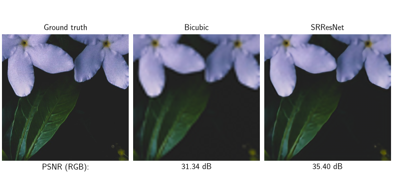
We apply DownsamplingMatlab to match the training physics. Note that only y is passed to the model, no physics is needed at inference. We compare against a standard bicubic interpolation baseline.

physics = dinv.physics.DownsamplingMatlab(factor=4, device=device)
psnr = dinv.metric.PSNR()

x = dinv.utils.load_example("div2k_valid_hr_0877.png", img_size=256, device=device)
y = physics(x)

with torch.no_grad():
    x_hat = model(y)
    x_bic = torch.nn.functional.interpolate(
        y, scale_factor=4, mode="bicubic", antialias=True
    )

dinv.utils.plot(
    {"Ground truth": x, "Bicubic": x_bic, "SRResNet": x_hat},
    subtitles=[
        "PSNR (RGB):",
        f"{psnr(x, x_bic).item():.2f} dB",
        f"{psnr(x, x_hat).item():.2f} dB",
    ],
    figsize=(8, 4),
    rescale_mode="clip",
)

2. Fine-tuning

SRResNet is fully trainable with Trainer. To demonstrate this, we fine-tune the pretrained model on a small subset of Urban100.

from torchvision.transforms import CenterCrop, Compose, ToTensor

torch.manual_seed(16)
hr_size = 64
dataset = dinv.datasets.Urban100HR(
    dinv.utils.get_cache_home() / "datasets" / "Urban100",
    download=True,
    transform=Compose([ToTensor(), CenterCrop(hr_size)]),
)

train_dataset, test_dataset = torch.utils.data.random_split(
    torch.utils.data.Subset(dataset, range(10)), (0.8, 0.2)
)

dataset_path = dinv.datasets.generate_dataset(
    train_dataset=train_dataset,
    test_dataset=test_dataset,
    physics=physics,
    device=device,
    save_dir=".",
    batch_size=1,
)

train_dataloader = torch.utils.data.DataLoader(
    dinv.datasets.HDF5Dataset(dataset_path, train=True), shuffle=True
)
test_dataloader = torch.utils.data.DataLoader(
    dinv.datasets.HDF5Dataset(dataset_path, train=False), shuffle=False
)

/local/jtachell/deepinv/deepinv/deepinv/datasets/datagenerator.py:600: UserWarning: Dataset ./dinv_dataset0.h5 already exists, this will close and overwrite the previous dataset.
  warn(
Dataset has been saved at ./dinv_dataset0.h5

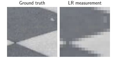
Visualise a data sample:

x, y = next(iter(test_dataloader))
dinv.utils.plot({"Ground truth": x, "LR measurement": y}, rescale_mode="clip")

We fine-tune the pretrained model.

Note

With only a handful of images and no regularisation, the model will overfit after the first few epochs and eval PSNR will decrease. We therefore load the best checkpoint after training. For a proper fine-tuning run, use a larger and more diverse dataset.

epochs = 10 if torch.cuda.is_available() else 1

trainer = dinv.Trainer(
    model=model,
    physics=physics,
    optimizer=torch.optim.Adam(model.parameters(), lr=1e-4),
    train_dataloader=train_dataloader,
    eval_dataloader=test_dataloader,
    epochs=epochs,
    losses=dinv.loss.SupLoss(metric=torch.nn.L1Loss()),
    metrics=dinv.metric.PSNR(),
    device=device,
    plot_images=False,
    show_progress_bar=False,
)

_ = trainer.train()
best_model = trainer.load_best_model()

/local/jtachell/deepinv/deepinv/deepinv/training/trainer.py:1337: UserWarning: non_blocking_transfers=True but DataLoader.pin_memory=False; set pin_memory=True to overlap host-device copies with compute.
  self.setup_train()
The model has 1549462 trainable parameters
Train epoch 0: TotalLoss=0.058, PSNR=23.404
Eval epoch 0: PSNR=31.542
Best model saved at epoch 1
Train epoch 1: TotalLoss=0.055, PSNR=24.172
Eval epoch 1: PSNR=31.181
Train epoch 2: TotalLoss=0.053, PSNR=24.378
Eval epoch 2: PSNR=30.941
Train epoch 3: TotalLoss=0.052, PSNR=24.714
Eval epoch 3: PSNR=27.647
Train epoch 4: TotalLoss=0.051, PSNR=24.798
Eval epoch 4: PSNR=26.771
Train epoch 5: TotalLoss=0.051, PSNR=24.601
Eval epoch 5: PSNR=28.251
Train epoch 6: TotalLoss=0.051, PSNR=24.812
Eval epoch 6: PSNR=29.374
Train epoch 7: TotalLoss=0.05, PSNR=24.959
Eval epoch 7: PSNR=30.17
Train epoch 8: TotalLoss=0.049, PSNR=24.859
Eval epoch 8: PSNR=31.167
Train epoch 9: TotalLoss=0.047, PSNR=25.602
Eval epoch 9: PSNR=31.135
Model, optimizer, epoch_start successfully loaded from checkpoint: 26-07-24-19:40:41/ckp_best.pth.tar

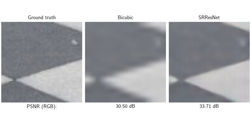
Plot a reconstruction from the best checkpoint:

x, y = x.to(device), y.to(device)
with torch.no_grad():
    x_ft = best_model(y)
    x_bic_ft = torch.nn.functional.interpolate(
        y, scale_factor=4, mode="bicubic", antialias=True
    )

dinv.utils.plot(
    {"Ground truth": x, "Bicubic": x_bic_ft, "SRResNet": x_ft},
    subtitles=[
        "PSNR (RGB):",
        f"{psnr(x, x_bic_ft).item():.2f} dB",
        f"{psnr(x, x_ft).item():.2f} dB",
    ],
    figsize=(8, 4),
    rescale_mode="clip",
)

References:

[1]

Christian Ledig, Lucas Theis, Ferenc Huszár, Jose Caballero, Andrew Cunningham, Alejandro Acosta, Andrew Aitken, Alykhan Tejani, Johannes Totz, Zehan Wang, and others. Photo-realistic single image super-resolution using a generative adversarial network. In Proceedings of the IEEE conference on computer vision and pattern recognition, 4681–4690. 2017.