3D diffraction PSF

This example provides a tour of 3D blur operators in the library. In particular, we show how to use Diffraction Blurs (Fresnel diffraction) to simulate fluorescence microscopes.

import torch
import deepinv as dinv

# First, let's load some test images.

dtype = torch.float32
device = dinv.utils.get_device()

# Next, set the global random seed from pytorch to ensure reproducibility of the example.
torch.manual_seed(0)
torch.cuda.manual_seed(0)

volume_data = (
    dinv.utils.load_np_url(
        "https://huggingface.co/datasets/deepinv/images/resolve/main/brainweb_t1_ICBM_1mm_subject_0.npy?download=true"
    )
    .flip(0)
    .unsqueeze(0)
    .unsqueeze(0)
)

x = volume_data / volume_data.max()
x = x.to(device)
b, c, d, h, w = x.size()

Selected GPU 0 with 21070.4375 MiB free memory

We are now ready to explore how to generate 3D blur operators for different microscopes.

3D convolutions

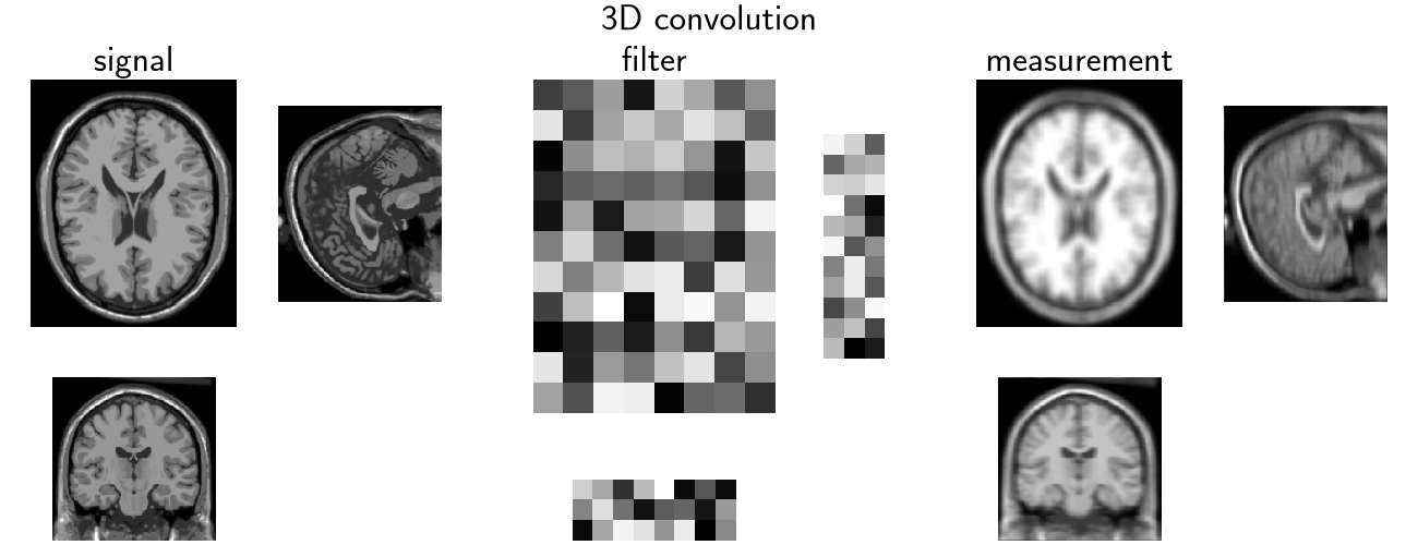
The class deepinv.physics.Blur implements convolution operations with kernels. It will automatically work for 3D images when given 5D torch.Tensor of size (B, C, D, H, W) for both the image and filter. Under the hood, the 3D convolutions are implemented through FFT. For instance, here is the convolution of a grayscale 3D image with a random grayscale filter:

filter_0 = torch.rand(1, 1, 3, 11, 8, device=device)
physics = dinv.physics.Blur(filter_0, device=device, padding="circular")
y = physics(x)

dinv.utils.plot_ortho3D(
    [x, filter_0, y],
    titles=["signal", "filter", "measurement"],
    suptitle="3D convolution",
    interpolation="nearest",
    figsize=(13, 5),
    tight=False,
    fontsize=24,
)

/local/jtachell/deepinv/deepinv/deepinv/physics/forward.py:500: UserWarning: Following torch.nn.Module's design, the 'device' attribute is deprecated and will be removed in a future version, i.e. doing `physics.device = device` will no longer work and throw an `AttributeError`. Use `physics.to(device)` instead.
  warnings.warn(
/local/jtachell/deepinv/deepinv/deepinv/utils/plotting.py:1267: UserWarning: This figure was using a layout engine that is incompatible with subplots_adjust and/or tight_layout; not calling subplots_adjust.
  fig.subplots_adjust(top=0.75)

Diffraction PSF generation

Advanced kernel generation methods are provided in the toolbox thanks to the class deepinv.physics.generator.PSFGenerator, that we used to construct PSF generators for different type of microscopes.

Widefield microscope PSF

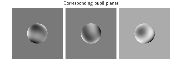
We implemented 3D diffraction blurs obtained using Fourier optics in deepinv.physics.generator.DiffractionBlurGenerator3D. Therein, the psf is defined through the pupil plane expanded in Zernike polynomials and the wave is propagated in the axial direction using the Fresnel approximation

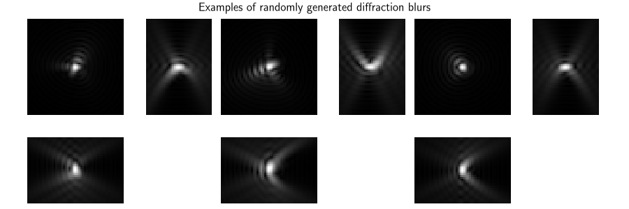
Let’s generate 3 different 3D diffraction blurs. First, we instantiate the generator:

from deepinv.physics.generator import DiffractionBlurGenerator3D

psf_size_XY = 51
psf_size_Z = 35
psf_size = (psf_size_Z, psf_size_XY, psf_size_XY)


diffraction_generator = DiffractionBlurGenerator3D(
    (psf_size_Z, psf_size_XY, psf_size_XY),
    stepz_pixel=2,
    device=device,
    dtype=dtype,
)

To generate new filters, it suffices to call the step() function. It takes as input the cutoff frequency fc and the wave number kb.

# For optician physicists: ``fc`` is the cutoff frequency, which should be below 0.25
# to respect Shannon's sampling theorem,  ``kb`` is the wave number, used for propagation
# in depth. Letting ``NA`` denote the numerical aperture, ``NI`` denote the index
# of refraction of the immersion medium and `lambda` denote the emission wavelength,
# the quantities are related through:
# `fc = (NA/lambda) * pixel_size`.
# `kb = (NI/lambda) * pixel_size`.


fc = 0.2
kb = 0.25
blurs = diffraction_generator.step(batch_size=3, fc=fc, kb=kb)

In this case, the step() function returns a dictionary containing the filters, their pupil function, Zernike coefficients and cut-off frequency:

print(blurs.keys())

dinv.utils.plot_ortho3D(
    [f[None] ** 0.5 for f in blurs["filter"]],
    suptitle="Examples of randomly generated diffraction blurs",
)

dinv.utils.plot(
    [
        f
        for f in torch.angle(blurs["pupil"][:, None])
        * torch.abs(blurs["pupil"][:, None])
    ],
    suptitle="Corresponding pupil planes",
)
print("Coefficients of the decomposition on Zernike polynomials")
print(blurs["coeff"])

• 
• 

dict_keys(['filter', 'pupil', 'coeff', 'fc'])
/local/jtachell/deepinv/deepinv/deepinv/utils/plotting.py:1302: UserWarning: This figure was using a layout engine that is incompatible with subplots_adjust and/or tight_layout; not calling subplots_adjust.
  plt.subplots_adjust(hspace=0.05, wspace=0.05)
/local/jtachell/deepinv/deepinv/deepinv/utils/plotting.py:449: UserWarning: This figure was using a layout engine that is incompatible with subplots_adjust and/or tight_layout; not calling subplots_adjust.
  fig.subplots_adjust(top=0.75)
Coefficients of the decomposition on Zernike polynomials
tensor([[[-0.0160,  0.0017,  0.0578, -0.0089,  0.0600, -0.0567,  0.0046,
          -0.0250]],

        [[-0.0392,  0.0006, -0.0610,  0.0743, -0.0712, -0.0380,  0.0690,
          -0.0289]],

        [[-0.0091,  0.0396, -0.0102,  0.0660,  0.0314,  0.0264, -0.0037,
           0.0203]]], device='cuda:0')

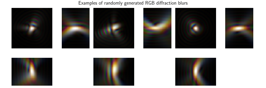
Generate physically realistic multi-colour diffraction PSFs by passing fc as a list to .step(). By default, step() accounts for wavelength-dependent diffraction (fc ∝ 1 / lambda) and rescales the Zernike coefficients so that all channels correspond to the same underlying physical aberrations.

lambdaR = 650
lambdaG = 550
lambdaB = 450
NA = 1.51
pixel_size = 50
fc = [NA * pixel_size / lambdaR, NA * pixel_size / lambdaG, NA * pixel_size / lambdaB]

diffraction_generator = DiffractionBlurGenerator3D(
    (psf_size_Z, psf_size_XY, psf_size_XY),
    stepz_pixel=2,
    device=device,
    dtype=dtype,
)

rgb_blurs = diffraction_generator.step(batch_size=3, fc=fc)

dinv.utils.plot_ortho3D(
    [f[None] ** 0.5 for f in rgb_blurs["filter"]],
    suptitle="Examples of randomly generated RGB diffraction blurs",
)

We provide a helper property to get the list of Zernike polynomials used in the decomposition:

zernike_polynomials = diffraction_generator.zernike_polynomials
print("Zernike polynomials used: \n", "\n ".join(zernike_polynomials))

# It is also possible to directly specify the Zernike decomposition.
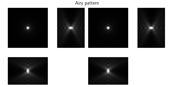
# For instance, if the pupil is null, the PSF is the Airy pattern.
# Notice that you then need to specify a cutoff frequenies with matching number of channels
n_zernike = len(
    zernike_polynomials
)  # number of Zernike coefficients in the decomposition
blurs = diffraction_generator.step(
    fc=0.2 * torch.ones(3, device=device),
    coeff=torch.zeros(2, 3, n_zernike, device=device),
)
dinv.utils.plot_ortho3D(
    [f**0.5 for f in blurs["filter"][:, None]],
    suptitle="Airy pattern",
)

Zernike polynomials used:
 Zernike(n = 2, m = 0) -- Defocus
 Zernike(n = 2, m = -2) -- Oblique Astigmatism
 Zernike(n = 2, m = 2) -- Vertical Astigmatism
 Zernike(n = 3, m = -1) -- Vertical Coma
 Zernike(n = 3, m = 1) -- Horizontal Coma
 Zernike(n = 3, m = -3) -- Vertical Trefoil
 Zernike(n = 3, m = 3) -- Oblique Trefoil
 Zernike(n = 4, m = 0) -- Primary Spherical

Finally, notice that you can activate the aberrations you want in the Noll nomenclature https://en.wikipedia.org/wiki/Zernike_polynomials#Noll’s_sequential_indices

diffraction_generator = DiffractionBlurGenerator3D(
    (psf_size_Z, psf_size_XY, psf_size_XY),
    fc=1 / 8,
    kb=0.25,
    stepz_pixel=2,
    zernike_index=(5, 6),
    device=device,
    dtype=dtype,
)
blurs = diffraction_generator.step(batch_size=3)

Confocal microscope PSF

We implemented the PSF of a confocal microscope in deepinv.physics.generator.ConfocalBlurGenerator3D. In fluorescence confocal microscopy, the light emitted by the sample is filtered through a pinhole to prevent the collection of out-of-focus light. The confocal intensity PSF can be expressed as

\[{\rm PSF}(r, z; \lambda_{ill}, \lambda_{coll}) = \vert h_{ill}(r, z; \lambda_{ill})\vert^2~ \left [ \vert h_{coll}(r, z; \lambda_{coll})\vert^2 \otimes_{2} D(r)\right ],\]

where \(h(r, z)\) is the amplitude PSF and \(D(r)\) is the detector intensity sensitivity distribution (here : one inside the confocal pinhole, 0 outside). ill coincides with illumination, while coll coincides with collection. \(\lambda\) coincides with the wavelength.

See Gu and Sheppard[1].

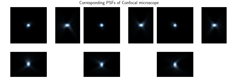
Here is a working example of a confocal microscope PSF imaging at three wavelengths.

from deepinv.physics.generator import ConfocalBlurGenerator3D

NI = 1.51  # refractive index of oil
angAper = 55  ##angular aperture in degrees
NA = NI * torch.sin(torch.deg2rad(torch.tensor([angAper]))).item()  # numerical aperture
lambda_ill = [450e-9, 550e-9, 650e-9]  # wavelength for illumniation in m
lambda_coll = [400e-9, 500e-9, 600e-9]  # wavelength for collection in m
pixelsize_XY = 70e-9  # in m
pixelsize_Z = 140e-9  # in m

generator = ConfocalBlurGenerator3D(
    psf_size=psf_size,
    NI=NI,
    NA=NA,
    lambda_ill=lambda_ill,
    lambda_coll=lambda_coll,
    pixelsize_XY=pixelsize_XY,
    pixelsize_Z=pixelsize_Z,
    num_channels=3,
)
blur_confocal = generator.step(batch_size=3)
psf_confocal = blur_confocal["filter"]


blur_coll = generator.generator_coll.step(
    batch_size=2, coeff=blur_confocal["coeff_coll"]
)
psf_coll = blur_coll["filter"]
# plot generated PSFs
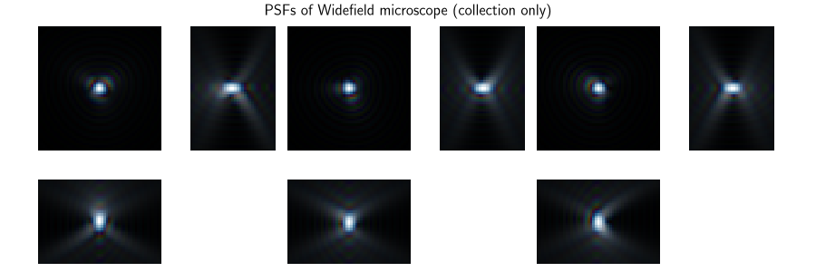
dinv.utils.plot_ortho3D(
    [psf[None] ** 0.5 for psf in psf_coll],
    suptitle="PSFs of Widefield microscope (collection only)",
)

dinv.utils.plot_ortho3D(
    [psf[None] ** 0.5 for psf in psf_confocal],
    suptitle="Corresponding PSFs of Confocal microscope",
)

• 
• 

References:

[1]

Min Gu and CJR Sheppard. Three-dimensional imaging in confocal fluorescent microscopy with annular lenses. Journal of Modern Optics, 38(11):2247–2263, 1991.