Random phase retrieval and reconstruction methods.

This example shows how to create a random phase retrieval operator and generate phaseless measurements from a given image. The example showcases 4 different reconstruction methods to recover the image from the phaseless measurements:

1. Gradient descent with random initialization;

2. Spectral methods;

3. Gradient descent with spectral methods initialization;

4. Gradient descent with PnP denoisers.

General setup

import deepinv as dinv
from pathlib import Path
import torch
import matplotlib.pyplot as plt
from deepinv.models import DRUNet
from deepinv.optim.data_fidelity import L2
from deepinv.optim.prior import PnP, ZeroPrior
from deepinv.optim import PGD
from deepinv.utils import load_example
from deepinv.utils.plotting import plot
from deepinv.optim.phase_retrieval import (
    correct_global_phase,
)
from deepinv.models.complex import to_complex_denoiser

BASE_DIR = Path(".")
RESULTS_DIR = BASE_DIR / "results"
# Set global random seed to ensure reproducibility.
torch.manual_seed(0)

device = dinv.utils.get_device()

Selected GPU 0 with 22698.4375 MiB free memory

Load image from the internet

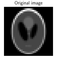
We use the standard test image “Shepp–Logan phantom”.

# Image size
img_size = 32
# The pixel values of the image are in the range [0, 1].
x = load_example(
    "SheppLogan.png",
    img_size=img_size,
    grayscale=True,
    resize_mode="resize",
    device=device,
)
print(x.min(), x.max())

tensor(0., device='cuda:0') tensor(0.7412, device='cuda:0')

Visualization

We use the customized plot() function in deepinv to visualize the original image.

plot(x, titles="Original image")

Signal construction

We use the original image as the phase information for the complex signal. The original value range is [0, 1], and we map it to the phase range [-pi/2, pi/2].

x_phase = torch.exp(1j * x * torch.pi - 0.5j * torch.pi)

# Every element of the signal should have unit norm.
assert torch.allclose(x_phase.real**2 + x_phase.imag**2, torch.tensor(1.0))

Measurements generation

Create a random phase retrieval operator with an oversampling ratio (measurements/pixels) of 5.0, and generate measurements from the signal with additive Gaussian noise.

# Define physics information
oversampling_ratio = 5.0
img_size = x.shape[1:]
m = int(oversampling_ratio * torch.prod(torch.tensor(img_size)))
n_channels = 1  # 3 for color images, 1 for gray-scale images

# Create the physics
physics = dinv.physics.RandomPhaseRetrieval(
    m=m,
    img_size=img_size,
    device=device,
)

# Generate measurements
y = physics(x_phase)

/local/jtachell/deepinv/deepinv/deepinv/physics/compressed_sensing.py:123: UserWarning: Complex modules are a new feature under active development whose design may change, and some modules might not work as expected when using complex tensors as parameters or buffers. Please file an issue at https://github.com/pytorch/pytorch/issues/new?template=bug-report.yml if a complex module does not work as expected.
  self.to(device=device, dtype=dtype)

Reconstruction with gradient descent and random initialization

First, we use the function deepinv.optim.L2 as the data fidelity function, and the class deepinv.optim.optim_iterators.GDIteration as the optimizer to run a gradient descent algorithm. The initial guess is a random complex signal.

data_fidelity = L2()
prior = ZeroPrior()
iterator = dinv.optim.optim_iterators.GDIteration()
# Parameters for the optimizer, including stepsize and regularization coefficient.
optim_params = {"stepsize": 0.06, "lambda": 1.0, "g_param": None}
num_iter = 1000

# Initial guess
x_phase_gd_rand = torch.randn_like(x_phase)

loss_hist = []

for _ in range(num_iter):
    res = iterator(
        {"est": (x_phase_gd_rand,), "cost": 0},
        cur_data_fidelity=data_fidelity,
        cur_prior=prior,
        cur_params=optim_params,
        y=y,
        physics=physics,
    )
    x_phase_gd_rand = res["est"][0]
    loss_hist.append(data_fidelity(x_phase_gd_rand, y, physics).cpu())

print("initial loss:", loss_hist[0])
print("final loss:", loss_hist[-1])
# Plot the loss curve
plt.plot(loss_hist)
plt.yscale("log")
plt.title("loss curve (gradient descent with random initialization)")
plt.show()

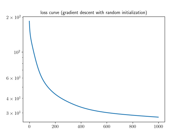
initial loss: tensor([184.1511])
final loss: tensor([27.5551])

Phase correction and signal reconstruction

The solution of the optimization algorithm x_est may be any phase-shifted version of the original complex signal x_phase, i.e., x_est = a * x_phase where a is an arbitrary unit norm complex number. Therefore, we use the function deepinv.optim.phase_retrieval.correct_global_phase to correct the global phase shift of the estimated signal x_est to make it closer to the original signal x_phase. We then use torch.angle to extract the phase information. With the range of the returned value being [-pi/2, pi/2], we further normalize it to be [0, 1]. This operation will later be done for all the reconstruction methods.

# correct possible global phase shifts
x_gd_rand = correct_global_phase(x_phase_gd_rand, x_phase)
# extract phase information and normalize to the range [0, 1]
x_gd_rand = torch.angle(x_gd_rand) / torch.pi + 0.5

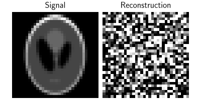
plot([x, x_gd_rand], titles=["Signal", "Reconstruction"], rescale_mode="clip")

Reconstruction with spectral methods

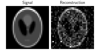
Spectral methods deepinv.optim.phase_retrieval.spectral_methods offers a good initial guess on the original signal. Moreover, deepinv.physics.RandomPhaseRetrieval uses spectral methods as its default reconstruction method A_dagger, which we can directly call.

# Spectral methods return a tensor with unit norm.
x_phase_spec = physics.A_dagger(y, n_iter=300)

Phase correction and signal reconstruction

# correct possible global phase shifts
x_spec = correct_global_phase(x_phase_spec, x_phase)
# extract phase information and normalize to the range [0, 1]
x_spec = torch.angle(x_spec) / torch.pi + 0.5
plot([x, x_spec], titles=["Signal", "Reconstruction"], rescale_mode="clip")

Reconstruction with gradient descent and spectral methods initialization

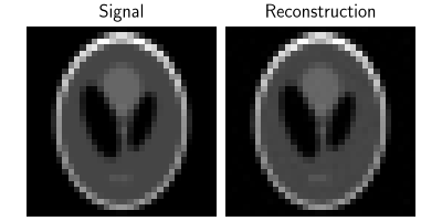
The estimate from spectral methods can be directly used as the initial guess for the gradient descent algorithm.

# Initial guess from spectral methods
x_phase_gd_spec = physics.A_dagger(y, n_iter=300)

loss_hist = []
for _ in range(num_iter):
    res = iterator(
        {"est": (x_phase_gd_spec,), "cost": 0},
        cur_data_fidelity=data_fidelity,
        cur_prior=prior,
        cur_params=optim_params,
        y=y,
        physics=physics,
    )
    x_phase_gd_spec = res["est"][0]
    loss_hist.append(data_fidelity(x_phase_gd_spec, y, physics).cpu())

print("intial loss:", loss_hist[0])
print("final loss:", loss_hist[-1])
plt.plot(loss_hist)
plt.yscale("log")
plt.title("loss curve (gradient descent with spectral initialization)")
plt.show()

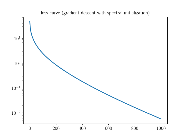
intial loss: tensor([47.4699])
final loss: tensor([0.0057])

Phase correction and signal reconstruction

# correct possible global phase shifts
x_gd_spec = correct_global_phase(x_phase_gd_spec, x_phase)
# extract phase information and normalize to the range [0, 1]
x_gd_spec = torch.angle(x_gd_spec) / torch.pi + 0.5
plot([x, x_gd_spec], titles=["Signal", "Reconstruction"], rescale_mode="clip")

Reconstruction with gradient descent and PnP denoisers

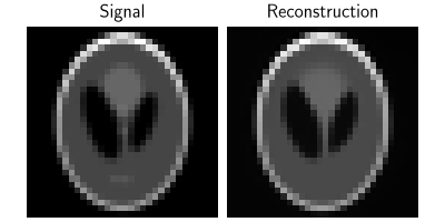
We can also use the Plug-and-Play (PnP) framework to incorporate denoisers as regularizers in the optimization algorithm. We use a deep denoiser as the prior, which is trained on a large dataset of natural images.

# Load the pre-trained denoiser
denoiser = DRUNet(
    in_channels=n_channels,
    out_channels=n_channels,
    pretrained="download",  # automatically downloads the pretrained weights, set to a path to use custom weights.
    device=device,
)
# The original denoiser is designed for real-valued images, so we need to convert it to a complex-valued denoiser for phase retrieval problems.
denoiser_complex = to_complex_denoiser(denoiser, mode="abs_angle")

# Algorithm parameters
data_fidelity = L2()
prior = PnP(denoiser=denoiser_complex)
stepsize = 0.3  # stepsize for the proximal gradient descent algorithm.
sigma_denoiser = 0.04  # noise level of the denoiser, used for the regularization parameter in the PnP algorithm.
max_iter = 100
early_stop = True
verbose = True

# Instantiate the algorithm class to solve the IP problem.
model = PGD(
    prior=prior,
    data_fidelity=data_fidelity,
    early_stop=early_stop,
    max_iter=max_iter,
    verbose=verbose,
    stepsize=stepsize,
    sigma_denoiser=sigma_denoiser,
)

# Run the algorithm
x_phase_pnp, metrics = model(y, physics, x_gt=x_phase, compute_metrics=True)

Phase correction and signal reconstruction

# correct possible global phase shifts
x_pnp = correct_global_phase(x_phase_pnp, x_phase)
# extract phase information and normalize to the range [0, 1]
x_pnp = torch.angle(x_pnp) / (2 * torch.pi) + 0.5
plot([x, x_pnp], titles=["Signal", "Reconstruction"], rescale_mode="clip")

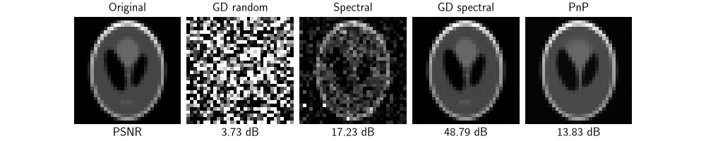
Overall comparison

We visualize the original image and the reconstructed images from the four methods. We further compute the PSNR (Peak Signal-to-Noise Ratio) scores (higher better) for every reconstruction and their cosine similarities with the original image (range in [0,1], higher better). In conclusion, gradient descent with random intialization provides a poor reconstruction, while spectral methods provide a good initial estimate which can later be improved by gradient descent to acquire the best reconstruction results. Besides, the PnP framework with a deep denoiser as the prior also provides a very good denoising results as it exploits prior information about the set of natural images.

subtitles = [
    "PSNR",
    f"{dinv.metric.PSNR()(x, x_gd_rand).item():.2f} dB",
    f"{dinv.metric.PSNR()(x, x_spec).item():.2f} dB",
    f"{dinv.metric.PSNR()(x, x_gd_spec).item():.2f} dB",
    f"{dinv.metric.PSNR()(x, x_pnp).item():.2f} dB",
]
plot(
    {
        "Original": x,
        "GD random": x_gd_rand,
        "Spectral": x_spec,
        "GD spectral": x_gd_spec,
        "PnP": x_pnp,
    },
    subtitles=subtitles,
    save_dir=RESULTS_DIR / "images",
    show=True,
    rescale_mode="clip",
)