Positron emission tomography (PET) in 2D

This demo shows how to define a non time-of-flight PET scanner, simulate measurements and reconstruct an image from them.

The PET forward model is defined as

\[y \sim \gamma \mathcal{P}\left(\frac{c \circ H(g*x) + b}{\gamma}\right)\]

where \(H \in \mathbb{R}_{+}^{m \times n}\) is the projection operator, \(g \in \mathbb{R}_{+}^{n}\) is a Gaussian blur kernel, \(x\in\mathbb{R}_{+}^{n}\) is the emission image, \(b \in \mathbb{R}_{+}^{m}\) is the (expected) background, \(\mathcal{P}\) denotes Poisson noise with gain \(\gamma > 0\), \(c=\exp(-H\mu)\in \mathbb{R}_{+}^{m}\) is an (optional) attenuation term with \(\mu \in \mathbb{R}_{+}^{n}\) an attenuation map (typically obtained through an auxiliary CT scan).

Note

This operator requires the parallelproj package to be installed. This in turn requires installing deepinv via pixi or conda, but not pypi/uv (as parallelproj is not currently available on pypi).

If you are working on a conda environment, you can install parallelproj as

conda install -c conda-forge parallelproj

If you are working on a pixi installation, simply do

pixi install -e full

which installs all optional dependencies.

Check the parallelproj documentation for more details: https://parallelproj.readthedocs.io/en/stable/.

import time

import matplotlib.pyplot as plt
import deepinv as dinv
from deepinv.physics import PET
from deepinv.utils.phantoms import generate_pet_phantom
import torch
import parallelproj
from array_api_compat import torch as torch_compat

Setup a minimal non-TOF PET projector

Here we define each pixel to have size \(3\times 3\) mm such that the total area to reconstruct is of size \(38.4\times 38.4\) cm which fits approximately a slice of a human chest.

The maximum achievable resolution (in high count settings) is typically proportional to the full-width at half maximum (FWHM) of the Gaussian blur kernel, which here is set to 4 mm.

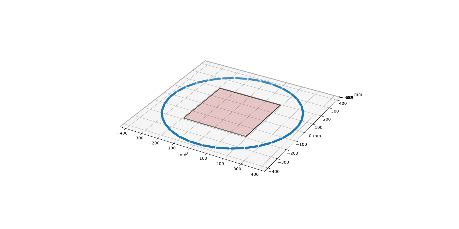
We use a PET scanner with a single ring of detectors, which is a polygon of 32 sides, with each side containing 16 detectors. This gives us a total of 32*16=512 detectors in total.

Tip

You can play with different geometries and voxel sizes to get a good grasp of the scanner geometry, and visualize it with physics.plot_geometry()

Note

In this example, we normalize the forward operator \(\|A\|=1\) (normalize=True) and the Poisson counts to be between 0 and 1 (normalize_counts=True), to simplify reconstruction. If you want to use the operator with real PET measurements, you will need to carefully handle the normalization. See also the unnormalized 3D PET example.

device = "cuda" if torch.cuda.is_available() else "cpu"
img_size = (128, 128)
voxel_size = (3, 3)

# number of sides of the polygon approximating a circle
num_sides = 32

# number of detectors per polygon side
num_lor_endpoints_per_side = 16

# choose a single ring for 2D
num_rings = 1

scanner = parallelproj.pet_scanners.DemoPETScannerGeometry(
    torch_compat,
    dev=device,
    num_rings=num_rings,
    num_sides=num_sides,
    num_lor_endpoints_per_side=num_lor_endpoints_per_side,
)

# gain of the device:
# higher gains are associated to lower dose and/or shorter acquisition times,
# while lower gains are associated to higher dose and/or longer acquisition times.
# larger gain -> more poisson noise -> harder reconstruction
gain = 0.001

# FWHM of the Gaussian blur kernel in mm
fwhm_data_mm = 4

physics = PET(
    device=device,
    voxel_size=voxel_size,
    fwhm_data_mm=fwhm_data_mm,
    scanner=scanner,
    img_size=img_size,
    normalize_counts=True,
    normalize=True,
    gain=gain,
)

physics.plot_geometry()

Define a phantom and attenuation map

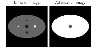
We define a 2D phantom and attenuation map, whose shape is the same as the phantom.

In practice, the attenuation is typically obtained with an auxiliary CT scan of the patient.

x, attenuation = generate_pet_phantom(img_size, device=device)

dinv.utils.plot(
    [x, attenuation], titles=["Emission image", "Attenuation image"], figsize=(8, 4)
)

Simulating measurements

The shape of measurements is approximately (B, 1, N, N/2) where N=num_lor_endpoints_per_side*num_sides is the number of detectors per ring. This provides one measurement for every possible Line of Response (LOR), or in other words ‘rays’, connecting two detectors in the scanner, which are arranged in a sinogram format, with the first axis corresponding to the angle of the ray and the second axis corresponding to the distance of the ray to the center of the field of view.

Tip

The size of measurements is independent of the chosen img_size

y = physics(x)

print(
    f"Measurements shape={tuple(y.shape)}, range=({y.min().item():.2f},{y.max().item():.2f})"
)

Measurements shape=(1, 1, 507, 256), range=(0.00,0.66)

Setting up background and attenuation

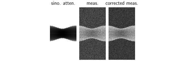
The attenuation term reduces the amount of signal measured in rays that go through highly attenuating regions, such as bones. This makes the reconstruction more challenging, but also more realistic.

In PET, we generally have access to a realization of the background, i.e., \(\tilde{s} \sim \mathcal{P}(s)\), which is a Poisson random variable with mean \(s\).

Both attenuation and background are stored as “physics parameters” which are patient dependent and can be updated via physics.update(...) or by passing them as kwargs in physics(x, ...), physics.A(x, ...) or physics.A_adjoint(y, ...).

Note

The attenuation is stored in the physics in sinogram space as \(\exp(-\mu)\) to speed up computations, but it can be provided either in image space, i.e., \(\mu\), to the physics, or in sinogram space, i.e., \(\exp(-\mu)\). The class figures out the attenuation space by comparing it to img_size.

expected_background = torch.ones_like(y) * x.max() * 0.05
background = physics.generate_background(expected_background)
physics.update(attenuation=attenuation, background=background)
y = physics(x)
y2 = y - background
dinv.utils.plot(
    [physics.attenuation, y, y2], ["sino. atten.", "meas.", "corrected meas."]
)

Backprojection and sensitivities

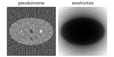
We backproject the data to visualize the sensitivity map of the scanner. The sensitivity map is defined as the back-projection of a sinogram of ones \(s = A^\top \mathbf{1}\), which corresponds to the number of rays intersecting each voxel.

Here we also obtain a simple linear least-squares reconstruction by using A_dagger.

with torch.no_grad():
    x_dag = physics.A_dagger(y - background)
    sensitivities = physics.A_adjoint(torch.ones_like(y))

print(f"Norm operator: {physics.compute_norm(x):.2f}")

dinv.utils.plot([x_dag, sensitivities], ["pseudoinverse", "sensitivities"])

Power iteration converged at iteration 12, ||A^T A||_2=0.99
Norm operator: 0.99

MLEM reconstruction

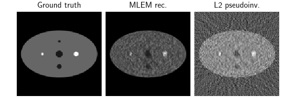
We run the standard MLEM reconstruction algorithm [1] to obtain a reconstructed emission volume.

The algorithm can be seen as a preconditioned gradient descent on the negative log-likelihood of the Poisson model:

\[x^{(k+1)} = x^{(k)} - P \nabla f(Ax^{(k)}+b,y)\]

where \(f\) is the Poisson data-fidelity term, \(P=\mathrm{diag}(\frac{x}{A^T\mathbf{1}})\) is a preconditioner and \(b\) is the background.

gain = physics.noise_model.gain
mlem_iter = 40


def _sync():
    if torch.device(device).type == "cuda":
        torch.cuda.synchronize()


nrmse = dinv.metric.NRMSE()


# With ``denormalize=True``, the likelihood is evaluated in the count domain.
# The background produced by PET is in the normalized measurement domain, so it
# must be divided by the gain as well.
data_fidelity = dinv.optim.PoissonLikelihood(
    gain=gain,
    bkg=background / gain,
    denormalize=True,
)
model_mlem = dinv.optim.MLEM(
    data_fidelity=data_fidelity,
    prior=None,
    max_iter=mlem_iter,
    custom_metrics={
        "nrmse": lambda _values, _x_prev, x_cur: nrmse(x_cur.unsqueeze(0), x).item()
    },
)

with torch.no_grad():
    _sync()
    start = time.perf_counter()
    x_mlem, metrics_mlem = model_mlem(
        y, physics, init=torch.ones_like(x), compute_metrics=True
    )
    _sync()
    mlem_time = time.perf_counter() - start

print(f"MLEM runtime: {mlem_time:.2f} s for {mlem_iter} iterations")

psnr = dinv.metric.PSNR(max_pixel=None)

psnr_mlem = psnr(x_mlem, x)
psnr_dag = psnr(x_dag, x)
nrmse_mlem = nrmse(x_mlem, x)
nrmse_dag = nrmse(x_dag, x)

dinv.utils.plot(
    [x, x_mlem, x_dag],
    ["Ground truth", f"MLEM ({mlem_iter} it.)", "L2 pseudoinv."],
    subtitles=[
        "Reference",
        f"PSNR: {psnr_mlem.item():.2f} dB\n" f"NRMSE: {100 * nrmse_mlem.item():.2f}%",
        f"PSNR: {psnr_dag.item():.2f} dB\n" f"NRMSE: {100 * nrmse_dag.item():.2f}%",
    ],
    rescale_mode="clip",
    vmin=0,
    vmax=x.max().item(),
    figsize=(8, 4),
    cbar=True,
)

MLEM runtime: 0.47 s for 40 iterations
/local/jtachell/deepinv/deepinv/deepinv/utils/plotting.py:493: UserWarning: set_ticklabels() should only be used with a fixed number of ticks, i.e. after set_ticks() or using a FixedLocator. Otherwise, ticks may be mislabeled.
  colbar.set_ticklabels(true_labels)
/local/jtachell/deepinv/deepinv/deepinv/utils/plotting.py:493: UserWarning: set_ticklabels() should only be used with a fixed number of ticks, i.e. after set_ticks() or using a FixedLocator. Otherwise, ticks may be mislabeled.
  colbar.set_ticklabels(true_labels)
/local/jtachell/deepinv/deepinv/deepinv/utils/plotting.py:493: UserWarning: set_ticklabels() should only be used with a fixed number of ticks, i.e. after set_ticks() or using a FixedLocator. Otherwise, ticks may be mislabeled.
  colbar.set_ticklabels(true_labels)
/local/jtachell/deepinv/deepinv/deepinv/utils/plotting.py:513: UserWarning: This figure was using a layout engine that is incompatible with subplots_adjust and/or tight_layout; not calling subplots_adjust.
  plt.subplots_adjust(hspace=0.2, wspace=0.2)

Accelerating MLEM with ordered subsets

One MLEM iteration evaluates the forward and adjoint operators using the complete PET acquisition. This can be slow when the scanner geometry and its measurements are large, especially in 3D.

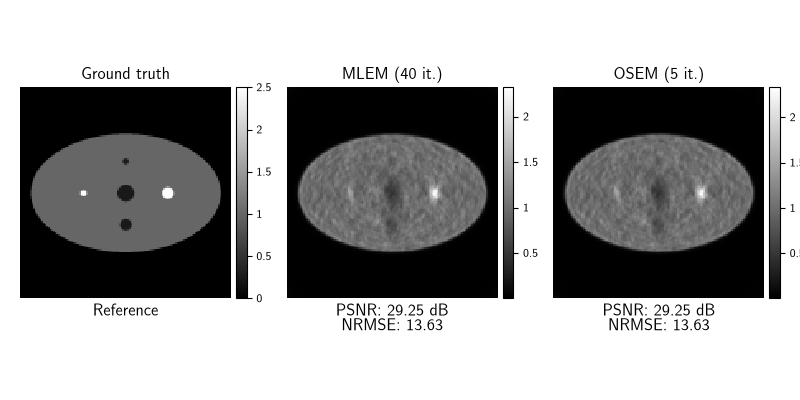
Ordered-Subsets Expectation-Maximization (OSEM) [2] partitions the measurements and the forward operator into \(L\) matching angular subsets indexed by \(l=1,\ldots,L\):

\[y = (y_1,\ldots,y_L), \qquad A = (A_1^\top,\ldots,A_L^\top)^\top.\]

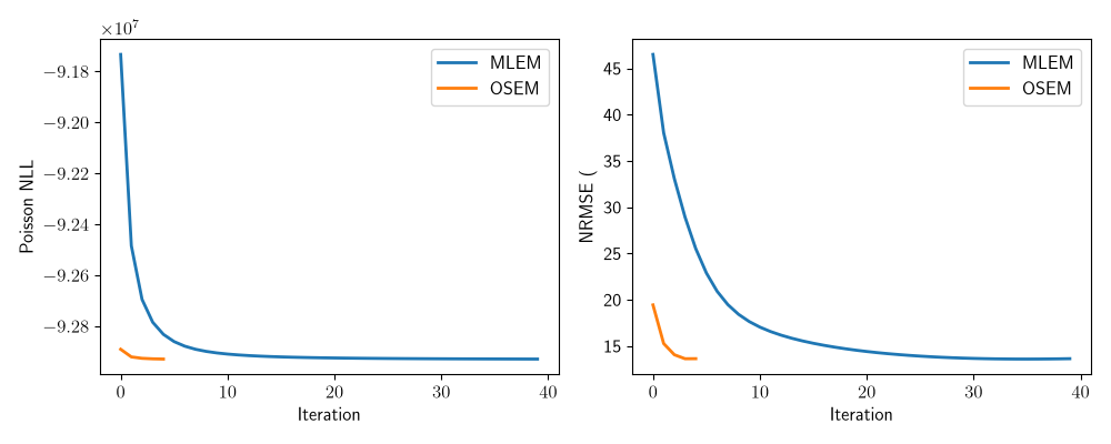
OSEM applies an EM update successively with each pair \((y_l,A_l)\). Each subset update is cheaper than a full MLEM iteration and updates the complete image, so OSEM generally reaches a useful reconstruction in fewer passes over the complete acquisition.

OSEM reconstruction

OSEM accepts the full measurements and physics and splits them internally. Alternatively, pre-split inputs can be created with deepinv.physics.split_measurements() and deepinv.physics.split_physics() and passed directly to deepinv.optim.OSEM.

osem_iter = 5
num_subsets = 8

model_osem = dinv.optim.OSEM(
    data_fidelity=data_fidelity,
    prior=None,
    max_iter=osem_iter,
    num_subsets=num_subsets,
    custom_metrics={
        "nrmse": lambda _values, _x_prev, x_cur: nrmse(x_cur.unsqueeze(0), x).item()
    },
)

with torch.no_grad():
    _sync()
    start = time.perf_counter()
    x_osem, metrics_osem = model_osem(
        y,
        physics,
        init=torch.ones_like(x),
        compute_metrics=True,
    )
    _sync()
    osem_time = time.perf_counter() - start

print(
    f"OSEM runtime: {osem_time:.2f} s "
    f"for {osem_iter} iterations "
    f"({num_subsets} subsets)"
)
print(f"Reconstruction speedup MLEM/OSEM: {mlem_time / osem_time:.2f}x")

psnr_osem = psnr(x_osem, x)
nrmse_osem = nrmse(x_osem, x)

dinv.utils.plot(
    [x, x_mlem, x_osem],
    [
        "Ground truth",
        f"MLEM ({mlem_iter} it.)",
        f"OSEM ({osem_iter} it.)",
    ],
    subtitles=[
        "Reference",
        f"PSNR: {psnr_mlem.item():.2f} dB\n" f"NRMSE: {100 * nrmse_mlem.item():.2f}%",
        f"PSNR: {psnr_osem.item():.2f} dB\n" f"NRMSE: {100 * nrmse_osem.item():.2f}%",
    ],
    rescale_mode="clip",
    vmin=0,
    vmax=x.max().item(),
    figsize=(8, 4),
    cbar=True,
)

# We also compare the Poisson objective and NRMSE after every iteration.
fig, axes = plt.subplots(1, 2, figsize=(10, 4))
axes[0].plot(metrics_mlem["cost"][0], label="MLEM")
axes[0].plot(metrics_osem["cost"][0], label="OSEM")
axes[0].set_xlabel("Iteration")
axes[0].set_ylabel("Poisson NLL")
axes[0].legend()

axes[1].plot([100 * v for v in metrics_mlem["nrmse"][0]], label="MLEM")
axes[1].plot([100 * v for v in metrics_osem["nrmse"][0]], label="OSEM")
axes[1].set_xlabel("Iteration")
axes[1].set_ylabel("NRMSE (%)")
axes[1].yaxis.set_major_formatter("{x:.0f}%")
axes[1].legend()
fig.tight_layout()

• 
• 

OSEM runtime: 1.24 s for 5 iterations (8 subsets)
Reconstruction speedup MLEM/OSEM: 0.38x
/local/jtachell/deepinv/deepinv/deepinv/utils/plotting.py:493: UserWarning: set_ticklabels() should only be used with a fixed number of ticks, i.e. after set_ticks() or using a FixedLocator. Otherwise, ticks may be mislabeled.
  colbar.set_ticklabels(true_labels)
/local/jtachell/deepinv/deepinv/deepinv/utils/plotting.py:493: UserWarning: set_ticklabels() should only be used with a fixed number of ticks, i.e. after set_ticks() or using a FixedLocator. Otherwise, ticks may be mislabeled.
  colbar.set_ticklabels(true_labels)
/local/jtachell/deepinv/deepinv/deepinv/utils/plotting.py:493: UserWarning: set_ticklabels() should only be used with a fixed number of ticks, i.e. after set_ticks() or using a FixedLocator. Otherwise, ticks may be mislabeled.
  colbar.set_ticklabels(true_labels)
/local/jtachell/deepinv/deepinv/deepinv/utils/plotting.py:513: UserWarning: This figure was using a layout engine that is incompatible with subplots_adjust and/or tight_layout; not calling subplots_adjust.
  plt.subplots_adjust(hspace=0.2, wspace=0.2)

What next?

Now that you master the basics of PET, you can go further by

• Check out the 3D PET example.

• Reconstructing PET with learning-based methods (PnP, diffusion, unrolled, etc.)

• Playing with the scanner setup: changing number of detectors, voxel size, etc.

References:

[1]

Lawrence A Shepp and Yehuda Vardi. Maximum likelihood reconstruction for emission tomography. IEEE Transactions on Medical Imaging, 1(2):113–122, 1982.

[2]

H.M. Hudson and R.S. Larkin. Accelerated image reconstruction using ordered subsets of projection data. IEEE Transactions on Medical Imaging, 13(4):601–609, December 1994. doi:10.1109/42.363108.