Multispectral demosaicing from raw sensor data

This example reconstructs a full-resolution multispectral image from raw snapshot mosaiced measurements using various reconstruction algorithms.

Snapshot multispectral cameras cover the sensor with a mosaic of spectral filters (multispectral filter array), so that each pixel records only one band. Demosaicing recovers every band at the full sensor resolution.

Demosaicing is a critical part of any image signal processing (ISP) pipeline, and using better algorithms results in higher quality images for downstream tasks.

We use raw oral-tissue data from the MODID dataset [1] acquired in-vivo for screening of oral diseases such as oral squamous cell carcinoma. See original data source. The data is unprocessed from an imec CMV2K-SSM4x4-VIS CMOS sensor covering 16 bands from 460 to 600 nm before any corrections. The sensor uses a sequential 4x4 MSFA i.e. 16 bands.

import torch
import deepinv as dinv

device = dinv.utils.get_device()

Selected GPU 0 with 19675.5 MiB free memory

Load and mosaic the raw data

We take sample 2 from MODID, hosted on the DeepInverse HuggingFace repository. You can explore further samples yourself from the original data source (licensed CC0 1.0). The file is a raw stream which we reshape to the pixel array of shape 1088x2048 and crop a 768x768 region of interest.

H, W = 1088, 2048
TILE = 4
CROP = 768
r0 = ((H - CROP) // 2 // TILE) * TILE
c0 = ((W - CROP) // 2 // TILE) * TILE

raw = torch.frombuffer(
    bytearray(dinv.utils.load_url(dinv.utils.get_image_url("modid.raw")).getvalue()),
    dtype=torch.float32,
).reshape(H, W)
raw = raw[r0 : r0 + CROP, c0 : c0 + CROP].to(device)  # 1, H, W where H=W=768

Unravel the mosaic into a 16-band image of shape (1, 16, 768, 768) and build the binary MSFA mask, which is 1 where a band is sampled and 0 elsewhere. Demosaicing is simply inpainting under this mask (see deepinv.physics.Demosaicing).

y = torch.zeros(1, 16, *raw.shape[-2:], device=device)
mask = torch.zeros_like(y)
for i in range(4):
    for j in range(4):
        c = i * 4 + j
        y[:, c, i::4, j::4] = raw[i::4, j::4]
        mask[:, c, i::4, j::4] = 1

y = y / y.max()  # normalise

physics = dinv.physics.Inpainting(img_size=mask.shape[1:], mask=mask, device=device)

Reconstruct with classical interpolation

As a classical baseline we fill the unsampled pixels of each band by Gaussian interpolation. This is a standard reconstruction used in many ISP pipelines.

class GaussianInterpolation(dinv.models.Reconstructor):
    def forward(self, y, physics, **kwargs):
        f = dinv.physics.functional.gaussian_blur(sigma=(1.5, 1.5), device=y.device)
        return torch.where(
            physics.mask > 0,
            y,
            dinv.physics.functional.conv2d(y, f, padding="replicate")
            / (
                dinv.physics.functional.conv2d(physics.mask, f, padding="replicate")
                + 1e-8
            ),
        )


model_classic = GaussianInterpolation().to(device)
with torch.no_grad():
    x_classic = model_classic(y, physics)

Reconstruct with total variation prior

We frame image reconstruction as an optimization problem and use the total variation prior to regularise the problem. We use a Proximal Gradient Descent (PGD) algorithm to solve the inverse problem. We use the classical interpolated reconstruction as a warm initialisation to speed up the optimization.

Note

We run 100 iterations on GPU, or 10 on CPU, which might not run to convergence. Increase it for better results.

model = dinv.optim.PGD(
    prior=dinv.optim.TVPrior(n_it_max=20),  # set larger on GPU
    data_fidelity=dinv.optim.L2(),
    stepsize=1.0,
    lambda_reg=0.01,
    max_iter=10 if dinv.utils.devices_equal(device, "cpu") else 100,
    custom_init=lambda y, physics: x_classic,
    verbose=True,
).to(device)

with torch.no_grad():
    x_tv = model(y, physics)

Visualise the results

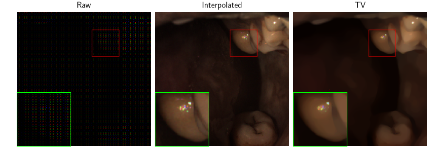
We plot the three bands closest to RGB: the full reconstruction has 16 bands. Interpolation shows chromatic errors at bright spots, an artefact of interpolating across bands. The TV reconstruction displays classic piecewise constant artifacts.

dinv.utils.plot(
    {
        "Raw": y[:, [3, 11, 12]],
        "Interpolated": x_classic[:, [3, 11, 12]],
        "TV": x_tv[:, [3, 11, 12]],
    },
    plot_inset=True,
    inset_loc=(0.0, 0.6),
    extract_loc=(0.56, 0.13),
    figsize=(9, 3),
)

What’s next?

We didn’t show any deep learning reconstruction methods in this example to keep the example lightweight. You can try out other types of reconstruction algorithms listed in the user guide. For example, you could try applying the Deep Image Prior [2][3]:

model = dinv.models.DeepImagePrior(
    dinv.models.ConvDecoder(img_size=mask.shape[1:]),
    img_size=(256, 4, 4),
    iterations=1000,
).to(device)

Instead of training models from scratch, you could also fine-tune a foundation model such as deepinv.models.RAM without ground truth as done in Wang and Davies[4].

References:

[1]

Sneha Chand, Karthik Namasivayam, Janak Dave, S. P. Preejith, Sadaksharam Jayachandran, and Mohanasankar Sivaprakasam. In-vivo non-contact multispectral oral disease image dataset with segmentation. Scientific Data, 11(1):1298, 2024.

[2]

Dmitry Ulyanov, Andrea Vedaldi, and Victor Lempitsky. Deep image prior. In Proceedings of the IEEE conference on computer vision and pattern recognition, 9446–9454. 2018.

[3]

Yunjin Park, Sukho Lee, Byeongseon Jeong, and Jungho Yoon. Joint demosaicing and denoising based on a variational deep image prior neural network. Sensors, 20(10):2970, 2020.

[4]

Andrew Wang and Mike Davies. Perspective-equivariant fine-tuning for multispectral demosaicing without ground truth. In Proceedings of the IEEE/CVF Conference on Computer Vision and Pattern Recognition (CVPR) Workshops. 2026.