

Note
New to DeepInverse? Get started with the basics with the 5 minute quickstart tutorial..
Reconstruct prospectively-undersampled raw multicoil MRI#
This example reconstructs real prospectively undersampled multicoil brain k-space from Yu et al.[1].
This demonstrates the performance of reconstruction algorithms in a deployment scenario rather than a typical simulated (retrospective) scenario. Here, it is impossible to compute full-reference metrics, since fully-sampled ground-truth does not exist.
We compare two types of reconstruction:
Deep learning, using a pretrained general model
deepinv.models.RAMfrom Terris et al.[2]Compressed sensing, using FISTA with a wavelet prior [3]
The data is stored in the raw ISMRMRD format.
Note
This example requires ismrmrd to load the data. Install it with pip install ismrmrd.
import torch
import deepinv as dinv

device = dinv.utils.get_device()
Selected GPU 0 with 8561.25 MiB free memory
Load the raw k-space#
The data is stored in the ISMRMRD format, as 3D multicoil kspace of shape (1, 2, N, D, H, W).
We inverse-FFT the fully-sampled readout/slice dimension D and take the middle slice to obtain a 2D multicoil kspace
for demonstration purposes.
dinv.datasets.download_archive(
    dinv.utils.get_image_url("t2_space_fs_sag_cs7_iso.h5"),
    dinv.utils.get_cache_home() / "mridata" / "prospective_t2.h5",
)

y = dinv.io.load_ismrmrd_raw(
    dinv.utils.get_cache_home() / "mridata" / "prospective_t2.h5", ifft_slice_dim=True
)
y = y[..., y.shape[-1] // 2, :, :].to(device)
File already downloaded: /local/jtachell/.cache/deepinv/mridata/prospective_t2.h5. Skipping...
Build the physics#
We recover the prospective sampling mask from the kspace zeros
We also estimate coil maps using ESPIRiT [4].
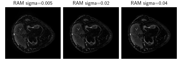
We estimate manually the noise level as sigma=0.02. Decreasing it increases the noise in the reconstruction, whereas
increasing it increases the smoothness in the reconstruction.
mask = (y != 0).any(1).any(1, keepdim=True).float()  # (1, 1, H, W)
coil_maps = dinv.physics.MultiCoilMRI.estimate_coil_maps(
    y, calib_size=24, espirit_crop=0.99
)  # (1, N, H, W) complex

physics = dinv.physics.MultiCoilMRI(
    mask=mask,
    coil_maps=coil_maps,
    device=device,
    noise_model=dinv.physics.GaussianNoise(sigma=0.02),
)
/local/jtachell/deepinv/deepinv/.pixi/envs/docs/lib/python3.12/site-packages/sigpy/config.py:27: UserWarning: Importing cupy.cuda.cudnn failed. For more details, see the error stack below:
No module named 'cupyx.cudnn'
  warnings.warn(
Baseline reconstructions#
As with any MRI problem, the baselines can be considered to be the zero-filled reconstruction, and the least-squares conjugate-gradient SENSE [5].
with torch.no_grad():
    x_zf = physics.A_adjoint(y)
    x_sense = physics.A_dagger(y)
Deep learning reconstruction with RAM#
Reconstruct Anything Model [2] was not trained on multicoil MRI physics, nor on axial knee MRI slices. Here, we therefore test its generalisability.
Note
ESPIRiT estimates coil maps with arbitrary phase per pixel, because the phases are unconstrained, leading to low spatial correlation.
Even though RAM is not trained on multicoil MRI, it performs better when the phase maps are also smooth. We use
physics.phase_correct_maps to constrain the phases to a smooth map, improving performance.
Tip
The sigma of the physics noise model controls the denoising strength. Here, we show a few options.
model = dinv.models.RAM(device=device, pretrained=True)

with torch.no_grad():
    coil_maps = physics.phase_correct_maps(x_zf)
    physics.update(coil_maps=coil_maps)

    # Although RAM is scale-equivariant, we bring y into friendlier scale (currently it's very small)
    x_ram = model(y / x_zf.max(), physics) * x_zf.max()

    physics.update(sigma=0.04)
    x_ram_high = model(y / x_zf.max(), physics) * x_zf.max()

    physics.update(sigma=0.005)
    x_ram_low = model(y / x_zf.max(), physics) * x_zf.max()

dinv.utils.plot(
    [x_ram_low, x_ram, x_ram_high],
    titles=["RAM sigma=0.005", "RAM sigma=0.02", "RAM sigma=0.04"],
)
Compressed sensing reconstruction#
We compare to compressed sensing reconstruction using the FISTA algorithm with a wavelet prior and L2 data fidelity.
Tip
The lambda_reg of the regularisation controls the regularisation strength. Here, we choose 2e-5.
We choose to use max 50 iterations for the demo. In practice, increase this to run to convergence.
prior = dinv.optim.WaveletPrior(
    level=3,
    wv=["db1", "db2", "db3", "db4", "db5", "db6", "db7", "db8"],
    p=1,
    device="cpu",
    clamp_min=0,
)

model = dinv.optim.FISTA(
    prior=prior,
    data_fidelity=dinv.optim.L2(),
    stepsize=0.1,
    lambda_reg=2e-5,
    early_stop=True,
    max_iter=50,
    verbose=True,
    custom_init=lambda y, physics: (physics.A_dagger(y), physics.A_dagger(y)),
    show_progress_bar=True,
)

x_fista = model(y, physics)
  0%|          | 0/50 [00:00<?, ?it/s]
  2%|▏         | 1/50 [00:00<00:05,  8.47it/s]
  4%|▍         | 2/50 [00:00<00:05,  9.07it/s]
  6%|▌         | 3/50 [00:00<00:05,  9.26it/s]
  8%|▊         | 4/50 [00:00<00:04,  9.37it/s]
 10%|█         | 5/50 [00:00<00:04,  9.42it/s]
 12%|█▏        | 6/50 [00:00<00:04,  9.46it/s]
 14%|█▍        | 7/50 [00:00<00:04,  9.49it/s]
 16%|█▌        | 8/50 [00:00<00:04,  9.50it/s]
 18%|█▊        | 9/50 [00:00<00:04,  9.50it/s]
 20%|██        | 10/50 [00:01<00:04,  9.51it/s]
 22%|██▏       | 11/50 [00:01<00:04,  9.51it/s]
 24%|██▍       | 12/50 [00:01<00:03,  9.51it/s]
 26%|██▌       | 13/50 [00:01<00:03,  9.51it/s]
 28%|██▊       | 14/50 [00:01<00:03,  9.51it/s]
 30%|███       | 15/50 [00:01<00:03,  9.51it/s]
 32%|███▏      | 16/50 [00:01<00:03,  9.51it/s]
 34%|███▍      | 17/50 [00:01<00:03,  9.52it/s]
 36%|███▌      | 18/50 [00:01<00:03,  9.51it/s]
 38%|███▊      | 19/50 [00:02<00:03,  9.51it/s]
 40%|████      | 20/50 [00:02<00:03,  9.48it/s]
 42%|████▏     | 21/50 [00:02<00:03,  9.50it/s]
 44%|████▍     | 22/50 [00:02<00:02,  9.50it/s]
 46%|████▌     | 23/50 [00:02<00:02,  9.50it/s]
 48%|████▊     | 24/50 [00:02<00:02,  9.50it/s]
 50%|█████     | 25/50 [00:02<00:02,  9.51it/s]
 52%|█████▏    | 26/50 [00:02<00:02,  9.51it/s]
 54%|█████▍    | 27/50 [00:02<00:02,  9.52it/s]
 56%|█████▌    | 28/50 [00:02<00:02,  9.52it/s]
 58%|█████▊    | 29/50 [00:03<00:02,  9.52it/s]
 60%|██████    | 30/50 [00:03<00:02,  9.51it/s]
 62%|██████▏   | 31/50 [00:03<00:01,  9.52it/s]
 64%|██████▍   | 32/50 [00:03<00:01,  9.52it/s]
 66%|██████▌   | 33/50 [00:03<00:01,  9.52it/s]
 68%|██████▊   | 34/50 [00:03<00:01,  9.51it/s]
 70%|███████   | 35/50 [00:03<00:01,  9.51it/s]
 72%|███████▏  | 36/50 [00:03<00:01,  9.51it/s]
 74%|███████▍  | 37/50 [00:03<00:01,  9.52it/s]
 76%|███████▌  | 38/50 [00:04<00:01,  9.52it/s]
 78%|███████▊  | 39/50 [00:04<00:01,  9.52it/s]
 80%|████████  | 40/50 [00:04<00:01,  9.51it/s]
 82%|████████▏ | 41/50 [00:04<00:00,  9.51it/s]
 84%|████████▍ | 42/50 [00:04<00:00,  9.50it/s]
 86%|████████▌ | 43/50 [00:04<00:00,  9.43it/s]
 88%|████████▊ | 44/50 [00:04<00:00,  9.44it/s]
 90%|█████████ | 45/50 [00:04<00:00,  9.42it/s]
 92%|█████████▏| 46/50 [00:04<00:00,  9.45it/s]
 94%|█████████▍| 47/50 [00:04<00:00,  9.48it/s]
 96%|█████████▌| 48/50 [00:05<00:00,  9.48it/s]
 98%|█████████▊| 49/50 [00:05<00:00,  9.48it/s]
100%|██████████| 50/50 [00:05<00:00,  9.50it/s]
100%|██████████| 50/50 [00:05<00:00,  9.48it/s]
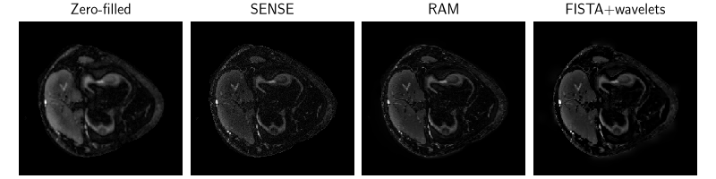
Plot the final comparison between methods:
dinv.utils.plot(
    [x_zf, x_sense, x_ram, x_fista],
    titles=["Zero-filled", "SENSE", "RAM", "FISTA+wavelets"],
)
- References:
Total running time of the script: (2 minutes 7.862 seconds)
