Multi-scale Plug-and-Play for Inpainting

Plug-and-Play (PnP) is known to be challenging to apply to certain inverse problems like inpainting. One way to overcome this is to use a multi-scale approach instead of the standard single-scale approach.

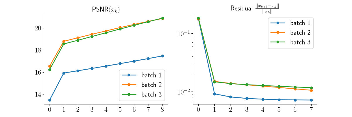
In this example, we show how to use multi-scale PnP and we benchmark it against a single-scale PnP baseline. Despite being slightly more computationally expensive, the results show that multi-scale PnP outputs significantly better reconstructions than the baseline.

For more details about multi-scale PnP, please refer to Laurent et al.[1].

import deepinv as dinv
import torch
from torch.utils.data import DataLoader
from torchvision import transforms

# For reproducilibity
torch.manual_seed(0)
torch.cuda.manual_seed_all(0)
torch.backends.cudnn.deterministic = True

# Select the device
device = dinv.utils.get_freer_gpu() if torch.cuda.is_available() else "cpu"

Selected GPU 0 with 9075.625 MiB free memory

The inpainting problem

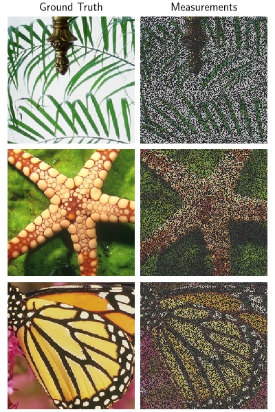
We start by defining the inpainting problem. We use images from the Set3C dataset and apply a random inpainting mask with 50% of the pixels missing to obtain the measurements. Additive white Gaussian noise is also added to the measurements to simulate a more realistic scenario.

# Create the dataset
img_size = (3, 32, 32) if torch.device(device).type == "cpu" else (3, 256, 256)
val_transform = transforms.Compose(
    [transforms.ToTensor(), transforms.CenterCrop(img_size[-2:])]
)
dataset = dinv.utils.load_dataset("set3c", transform=val_transform)
dataloader = DataLoader(dataset, batch_size=3, shuffle=False)

# Create the physics operator
noise_model = dinv.physics.GaussianNoise(sigma=0.1)
physics = dinv.physics.Inpainting(
    img_size=img_size, mask=0.5, noise_model=noise_model, device=device
)

# Display the ground truths and the measurements
x = next(iter(dataloader)).to(device)
y = physics(x)
dinv.utils.plot([x, y], ["Ground Truth", "Measurements"])

Single-scale and multi-scale PnP models

The multi-scale PnP model can be understood as a combination of multiple single-scale PnP models operating at different scales. Here, we use two scales: the fine scale corresponding to the scale of the original image, and a coarse scale corresponding to the fine scale downsampled by a factor of 2.

A base reconstruction is done in the coarse scale using the single-scale PnP model operating in the coarse scale, using a downsampled version of the measurements and of the physics operator. This base reconstruction is then upsampled in the fine scale and used as the initialization for the single-scale PnP model operating in the fine scale. In the end, this latter model outputs the final reconstruction of the multi-scale PnP model.

For both models, we use a L2 data fidelity term and a pre-trained DRUNet denoiser.

# Define the parameters shared between the single- and multi-scale PnP models
data_fidelity = dinv.optim.data_fidelity.L2()
denoiser = dinv.models.DRUNet(pretrained="download", device=device)
prior = dinv.optim.prior.PnP(denoiser=denoiser)
pgd_kwargs = {
    "prior": prior,
    "data_fidelity": data_fidelity,
    "early_stop": False,
    "params_algo": {"stepsize": 1.0, "g_param": 0.05},
}


# Define the initialization scheme for the multi-scale PnP model
def init_ms(y: torch.Tensor, physics: dinv.physics.Physics) -> dict:
    # Create a multi-scale physics from the single-scale physics
    physics_ms = dinv.physics.to_multiscale(
        physics, y.shape[1:], factors=(2,), device=device
    )

    # Set the working scale to the coarse scale
    physics_ms.set_scale(1)

    # Compute the measurements in the coarse scale
    y_coarse = physics_ms.downsample_measurement(y)

    # Define the single-scale PnP model operating at the coarse scale
    model_cs = dinv.optim.PGD(max_iter=16, **pgd_kwargs)

    # Reconstruct the image in the coarse scale
    x_coarse = model_cs(y, physics_ms)

    # Compute the base reconstruction in the fine scale
    x_fine = physics_ms.upsample(x_coarse)

    # Use the base reconstruction in the fine scale as the initialization for
    # the PnP model operating at the fine scale
    return {"est": [x_fine]}


# Define the single-scale PnP model operating at the fine scale and the
# multi-scale PnP model
model_fs = dinv.optim.PGD(max_iter=24, **pgd_kwargs)
model_ms = dinv.optim.PGD(max_iter=8, custom_init=init_ms, **pgd_kwargs)

Results

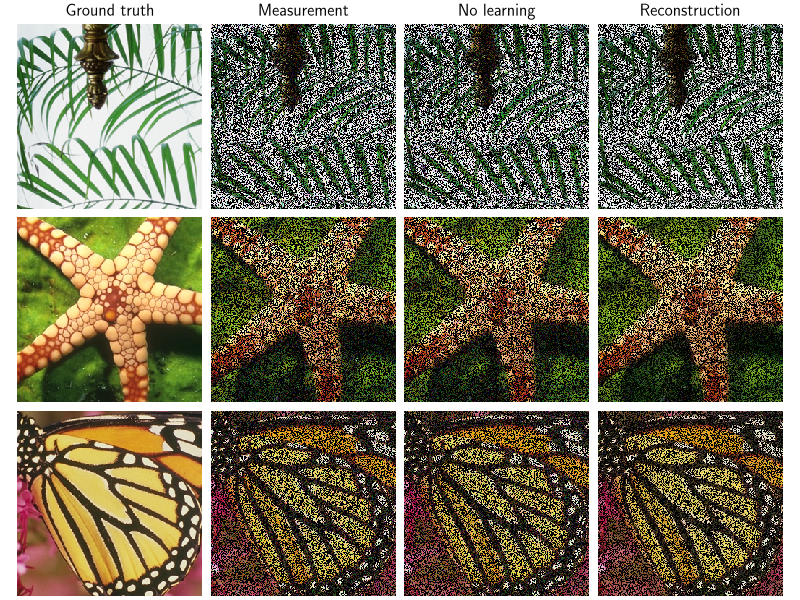
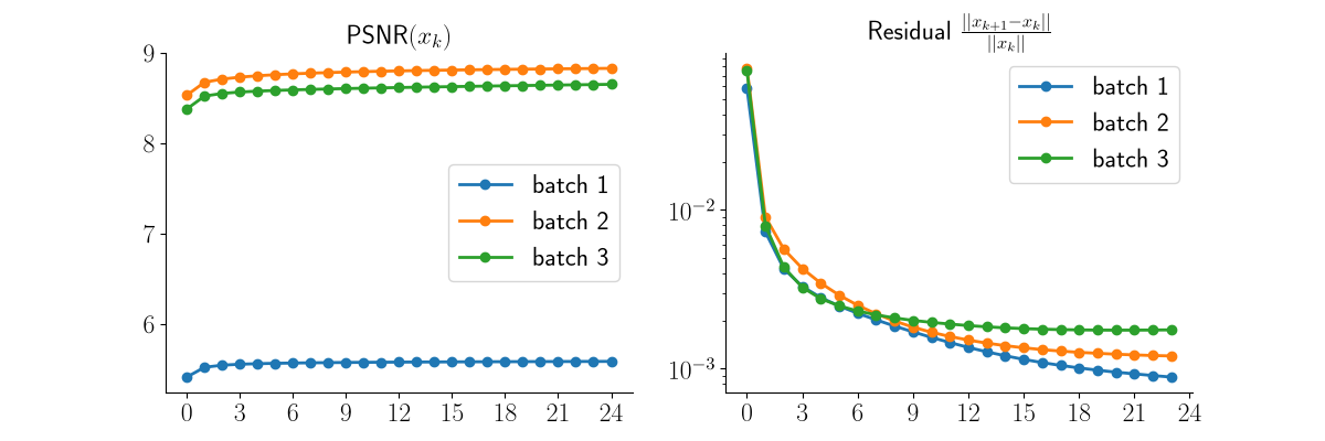
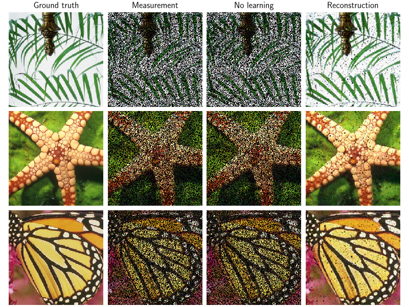
We benchmark the single-scale and multi-scale PnP models on the imaging problem and we see that contrary to the single-scale PnP model which barely improves the quality of the input image (top), the multi-scale PnP model produces a significantly better reconstruction which shows the benefit of the multi-scale approach (bottom).

# Set the model to evaluation mode since we do not require training.
# run the model on chosen dataset
test_kwargs = {
    "test_dataloader": dataloader,
    "physics": physics,
    "metrics": [dinv.metric.PSNR()],
    "device": device,
    "online_measurements": True,
    "plot_images": True,
    "plot_convergence_metrics": True,
    "verbose": True,
}

# Benchmark single-scale PnP
dinv.test(model=model_fs, **test_kwargs)

# Benchmark multi-scale PnP
dinv.test(model=model_ms, **test_kwargs)

• 
• 
• 
• 

/local/jtachell/deepinv/deepinv/deepinv/training/trainer.py:542: UserWarning: Update progress bar frequency of 1 may slow down training on GPU. Consider setting freq_update_progress_bar > 1.
  warnings.warn(

  0%|          | 0/1 [00:00<?, ?it/s]
Test:   0%|          | 0/1 [00:00<?, ?it/s]
Test:   0%|          | 0/1 [00:01<?, ?it/s, PSNR=7.69, PSNR no learning=7.44]
Test: 100%|██████████| 1/1 [00:01<00:00,  1.38s/it, PSNR=7.69, PSNR no learning=7.44]
Test: 100%|██████████| 1/1 [00:01<00:00,  1.38s/it, PSNR=7.69, PSNR no learning=7.44]
Test results:
PSNR no learning: 7.444 +- 1.436
PSNR: 7.692 +- 1.489

  0%|          | 0/1 [00:00<?, ?it/s]
Test:   0%|          | 0/1 [00:00<?, ?it/s]
Test:   0%|          | 0/1 [00:00<?, ?it/s, PSNR=19.7, PSNR no learning=7.44]
Test: 100%|██████████| 1/1 [00:00<00:00,  1.18it/s, PSNR=19.7, PSNR no learning=7.44]
Test: 100%|██████████| 1/1 [00:00<00:00,  1.18it/s, PSNR=19.7, PSNR no learning=7.44]
Test results:
PSNR no learning: 7.444 +- 1.436
PSNR: 19.738 +- 1.604

{'PSNR no learning': 7.444494883219401, 'PSNR no learning_std': 1.4360725485537766, 'PSNR': 19.738079071044922, 'PSNR_std': 1.6043075200947665, 'runtime': 0.8445472778985277, 'peak_gpu_memory_usage': 0.5324225425720215}

References:

[1]

Nils Laurent, Julián Tachella, Elisa Riccietti, and Nelly Pustelnik. Multilevel plug-and-play image restoration. IEEE Transactions on Computational Imaging, 2025.