Physics#
- class deepinv.physics.Physics(A=lambda x, **kwargs: ..., noise_model=None, sensor_model=lambda x: ..., solver='gradient_descent', max_iter=50, tol=1e-4, **kwargs)[source]#
Bases:
ModuleParent class for forward operators
It describes the general forward measurement process
\[y = \noise{\forw{x}}\]where \(x\) is an image of \(n\) pixels, \(y\) is the measurements of size \(m\), \(A:\xset\mapsto \yset\) is a deterministic mapping capturing the physics of the acquisition and \(N:\yset\mapsto \yset\) is a stochastic mapping which characterizes the noise affecting the measurements.
- Parameters:
A (Callable) – forward operator function which maps an image to the observed measurements \(x\mapsto y\).
noise_model (deepinv.physics.NoiseModel, Callable) – function that adds noise to the measurements \(\noise{z}\). See the noise module for some predefined functions.
sensor_model (Callable) – function that incorporates any sensor non-linearities to the sensing process, such as quantization or saturation, defined as a function \(\sensor{z}\), such that \(y=\sensor{\noise{\forw{x}}}\). By default, the
sensor_modelis set to the identity \(\sensor{z}=z\).max_iter (int) – If the operator does not have a closed form pseudoinverse, the gradient descent algorithm is used for computing it, and this parameter fixes the maximum number of gradient descent iterations.
tol (float) – If the operator does not have a closed form pseudoinverse, the gradient descent algorithm is used for computing it, and this parameter fixes the absolute tolerance of the gradient descent algorithm.
solver (str) – least squares solver to use. Only gradient descent is available for non-linear operators.
- A(x, **kwargs)[source]#
Computes forward operator \(y = A(x)\) (without noise and/or sensor non-linearities)
- Parameters:
x (torch.Tensor,list[torch.Tensor]) – signal/image
- Returns:
(
torch.Tensor) clean measurements
- A_dagger(y, x_init=None)[source]#
Computes an inverse as:
\[x^* \in \underset{x}{\arg\min} \quad \|\forw{x}-y\|^2.\]This function uses gradient descent to find the inverse. It can be overwritten by a more efficient pseudoinverse in cases where closed form formulas exist.
- Parameters:
y (torch.Tensor) – a measurement \(y\) to reconstruct via the pseudoinverse.
x_init (None, torch.Tensor) – initial guess for the reconstruction. If
None(default) it is set to the adjoint of the forward operator (it it exists) applied to the measurements \(y\), i.e., \(x_0 = A^{\top}y\).
- Returns:
(
torch.Tensor) The reconstructed image \(x\).
- A_vjp(x, v)[source]#
Computes the product between a vector \(v\) and the Jacobian of the forward operator \(A\) evaluated at \(x\), defined as:
\[A_{vjp}(x, v) = \left. \frac{\partial A}{\partial x} \right|_x^\top v.\]By default, the Jacobian is computed using automatic differentiation.
- Parameters:
x (torch.Tensor) – signal/image.
v (torch.Tensor) – vector.
- Returns:
(
torch.Tensor) the VJP product between \(v\) and the Jacobian.
- __mul__(other)[source]#
Concatenates two forward operators \(A = A_1\circ A_2\) via the mul operation
The resulting operator keeps the noise and sensor models of \(A_1\).
- Parameters:
other (deepinv.physics.Physics) – Physics operator \(A_2\)
- Returns:
(
deepinv.physics.Physics) concatenated operator
- clone()[source]#
Clone the forward operator by performing deepcopy to copy all attributes to new memory.
This method should be favored to
copy.deepcopyas it works even in the presence oftorch.Generatorobjects. Seethis issue <https://github.com/pytorch/pytorch/issues/43672>for more details.
- compute_norm(x, verbose=True)[source]#
Computes an estimate of the operator norm of the forward operator \(\|A\|_2\) at point
x.This function uses the power method to compute the operator norm.
- Parameters:
x (torch.Tensor) – input tensor used to estimate the norm.
verbose (bool) – if
True, prints the estimated norm.
- Returns:
(
torch.Tensor) estimated operator norm.
- forward(x, **kwargs)[source]#
Computes forward operator
\[y = N(A(x), \sigma)\]- Parameters:
x (torch.Tensor, list[torch.Tensor]) – signal/image
- Returns:
(
torch.Tensor) noisy measurements
- noise(x, **kwargs)[source]#
Incorporates noise into the measurements \(\tilde{y} = N(y)\)
- Parameters:
x (torch.Tensor) – clean measurements
noise_level (None, float) – optional noise level parameter
- Returns:
noisy measurements
- Return type:
- sensor(x)[source]#
Computes sensor non-linearities \(y = \eta(y)\)
- Parameters:
x (torch.Tensor,list[torch.Tensor]) – signal/image
- Returns:
(
torch.Tensor) clean measurements
- set_ls_solver(solver, max_iter=None, tol=None)[source]#
Change default solver for computing the least squares solution:
\[x^* \in \underset{x}{\arg\min} \quad \|\forw{x}-y\|^2.\]- Parameters:
solver (str) – solver to use. If the physics are non-linear, the only available solver is
'gradient_descent'. For linear operators, the options are'CG','lsqr','BiCGStab'and'minres'(seedeepinv.optim.linear.least_squares()for more details).max_iter (int) – maximum number of iterations for the solver.
tol (float) – relative tolerance for the solver, stopping when \(\|A(x) - y\| < \text{tol} \|y\|\).
- set_noise_model(noise_model, **kwargs)[source]#
Sets the noise model
- Parameters:
noise_model (Callable) – noise model
- stack(other)[source]#
Stacks two forward operators \(A(x) = \begin{bmatrix} A_1(x) \\ A_2(x) \end{bmatrix}\)
The measurements produced by the resulting model are
deepinv.utils.TensorListobjects, where each entry corresponds to the measurements of the corresponding operator.Returns a
deepinv.physics.StackedPhysicsobject.See Combining Physics for more information.
- Parameters:
other (deepinv.physics.Physics) – Physics operator \(A_2\)
- Returns:
(
deepinv.physics.StackedPhysics) stacked operator
Examples using Physics:#

Imaging inverse problems with adversarial networks




Reconstruct real CT sinograms with the 2DeteCT benchmark

Low-dose CT with ASTRA backend and Total-Variation (TV) prior


Reconstruct accelerated non-Cartesian breast MRI acquisition data


Reconstruct undersampled k-space for cardiac and brain MRI
Reconstruct prospectively-undersampled raw multicoil MRI


3D denoising of brain MRI with wavelet and TV priors


Reconstructing an image using the deep image prior.

Expected Patch Log Likelihood (EPLL) for Denoising and Inpainting

Patch priors for limited-angle computed tomography

Poisson Inverse Problems with Maximum-Likelihood Expectation-Maximization (MLEM)


Poisson-Gaussian Denoising with the Generalized Anscombe Transform


Spectral Methods for Non-Circular Deblurring with Liu-Jia Padding



Random phase retrieval and reconstruction methods.


Pattern Ordering in a Compressive Single Pixel Camera


PnP with custom optimization algorithm (Primal-Dual Condat-Vu)

Plug-and-Play algorithm with Mirror Descent for Poisson noise inverse problems.
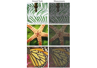

Regularization by Denoising (RED) for Super-Resolution.
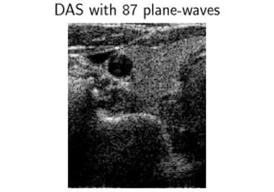
In-vivo ultrafast ultrasound reconstruction with Plug-and-Play


Using state-of-the-art diffusion models from HuggingFace Diffusers with DeepInverse

Building your diffusion posterior sampling method using SDEs


Flow-Matching for posterior sampling and unconditional generation
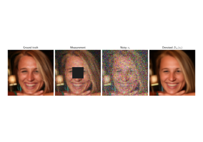
Noisy data-fidelity terms for diffusion posterior sampling


Self-supervised MRI reconstruction with Artifact2Artifact


Self-supervised learning with Equivariant Imaging for MRI.

Self-supervised learning with Equivariant Splitting


Self-supervised learning from incomplete measurements of multiple operators.

Self-supervised denoising with the Neighbor2Neighbor loss.


Self-supervised denoising with the Generalized R2R loss.


Self-supervised learning with measurement splitting


Deep Equilibrium (DEQ) algorithms for image deblurring

Learned Iterative Soft-Thresholding Algorithm (LISTA) for compressed sensing


Reducing the memory and computational complexity of unfolded network training

Unfolded Chambolle-Pock for constrained image inpainting
