Tour of ultrafast ultrasound in DeepInverse

This example presents the plane-wave ultrafast ultrasound forward physics (deepinv.physics.UltrasoundPlaneWave) available in DeepInverse for pulse-echo imaging problems.

We demonstrate simulating raw RF ultrasound data with/without a pulse-echo, beamforming with delay-and-sum (i.e. the adjoint), both for single-plane-wave imaging and >1 plane waves (i.e. coherent plane-wave compounding, or CPWC).

import math

import torch
import matplotlib.pyplot as plt
import deepinv as dinv

device = dinv.utils.get_device()

Selected GPU 0 with 6908.25 MiB free memory

1. The acquisition setup

As a first step, let’s simulate the following pulse-echo experiment: A 64-element linear array at 0.3 mm pitch fires 11 plane waves spread over \(\pm 12^\circ\). The center frequency of the array is 5 MHz and the speed of sound is 1540 m/s. The region to image is given in meters: 5 to 40 mm deep, 24 mm wide. The resolution of the image grid is set to lam / 6 axially (to fullfill Nyquist requirements) and lam / 1.5 laterally.

n_elements, pitch = 64, 3e-4
element_x = (torch.arange(n_elements) - (n_elements - 1) / 2) * pitch
element_positions = torch.stack([element_x, torch.zeros(n_elements)], dim=-1).to(device)
aperture = element_x.max() - element_x.min()

angles = torch.linspace(math.radians(-12.0), math.radians(12.0), 11, device=device)

sound_speed, center_frequency, sampling_frequency = 1540.0, 5e6, 20e6
wavelength = sound_speed / center_frequency

depth_min, depth_max, width = 5e-3, 40e-3, 24e-3
pixel_size = (wavelength / 6, wavelength / 1.5)
pixel_origin = (depth_min, -width / 2)
img_size = (
    round((depth_max - depth_min) / pixel_size[0]),
    round(width / pixel_size[1]),
)
print(f"Image size: {img_size}")

Image size: (682, 117)

2. The pulse-echo impulse response

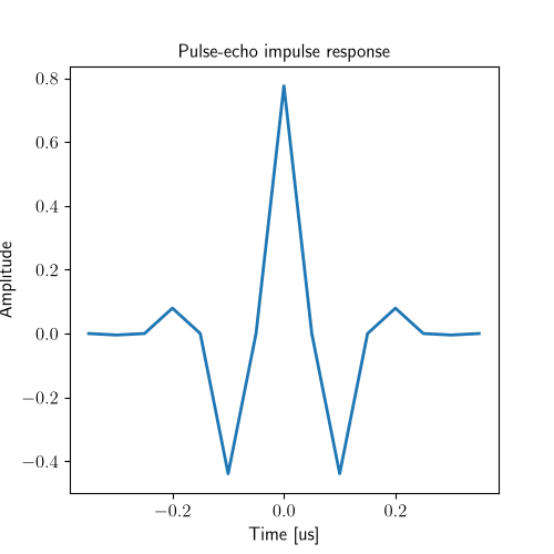
In order to account for the physics of a transducer element, we simulate a typical pulse-echo impulse response as a Gaussian-modulated pulse with a given fractional bandwidth and center frequency. This pulse-echo impulse response models the response of a transducer element i.e. how acoustical signals are transformed to electrical signals and vice-versa.

fractional_bandwidth = 0.8
sigma_t = math.sqrt(2 * math.log(2)) / (
    math.pi * fractional_bandwidth * center_frequency
)
n_half = math.ceil(3.5 * sigma_t * sampling_frequency)
t_pulse = torch.arange(-n_half, n_half + 1, device=device) / sampling_frequency
pulse = torch.exp(-(t_pulse**2) / (2 * sigma_t**2)) * torch.cos(
    2 * math.pi * center_frequency * t_pulse
)
pulse = pulse / torch.linalg.norm(pulse)
fig, ax = plt.subplots(1, 1, figsize=(5, 5))
ax.plot(t_pulse.cpu() * 1e6, pulse.cpu())
ax.set_title("Pulse-echo impulse response")
ax.set_ylabel("Amplitude")
ax.set_xlabel("Time [us]")

Text(0.5, 24.96281171085858, 'Time [us]')

The number of samples recorded by the transducer elements corresponds to the time taken by the ultrasound wave to travel the longest path of our experiment. The first term corresponds to the longest path in transmit (at most hypot(x, z) over all angles) and the second term to the longest path in receive (extreme left of the transducer to the lower right corner). The pulse length is added since the convolution spreads each echo in time.

longest_path = math.hypot(depth_max, width / 2) + math.hypot(
    depth_max, (width + aperture) / 2
)
n_samples = math.ceil(longest_path / sound_speed * sampling_frequency) + pulse.numel()

3. Defining the forward operator

deepinv.physics.UltrasoundPlaneWave gathers the grid to reconstruct on (img_size, pixel_size, pixel_origin), the sequence (angles), the probe (element_positions, sampling_frequency, sound_speed, pulse) and the beamforming settings (f_number, receive_apod_window).

physics = dinv.physics.UltrasoundPlaneWave(
    img_size=img_size,
    angles=angles,
    element_positions=element_positions,
    n_samples=n_samples,
    sampling_frequency=sampling_frequency,
    sound_speed=sound_speed,
    pixel_size=pixel_size,
    pixel_origin=pixel_origin,
    t0=0.0,
    pulse=pulse,
    normalize=False,
    device=device,
    f_number=1.5,
    receive_apod_window="hann",
)

4. Simulating per-channel raw data

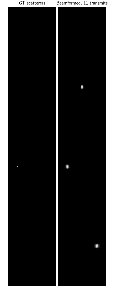
We simulate the per-channel raw RF data using the operator defined before. To do so, we consider a reflectivity map x composed of 3 points located at (0, 15mm), (-7.5mm, 25mm) and (7.5mm, 35mm).

x = torch.zeros(1, 1, *img_size, device=device)
grid = physics.pixel_grid
spots = []
for depth_mm, lateral_mm in ((15.0, 0.0), (25.0, -7.5), (35.0, 7.5)):
    position = torch.tensor([lateral_mm, depth_mm], device=grid.device) * 1e-3
    distance = torch.linalg.vector_norm(grid - position, dim=-1)
    ind_dist = int(distance.argmin())
    ind_x = ind_dist // img_size[1]
    ind_z = ind_dist % img_size[1]
    x[0, 0, ind_x, ind_z] = 1.0
    spots.append((ind_x, ind_z))

y = physics(x)

y_bmode = dinv.utils.bmode(y, dim=-1, amplitude_floor_db=-40.0, normalize=True)

dinv.utils.plot(
    y_bmode[:, :, 0],
    titles=[r"Channel data, transmit at $-12^\circ$"],
    figsize=(20, 4),
)

5. Beamforming with the adjoint

We build an estimate of the reflectivity map (the traditional DAS image) by applying the adjoint operator to the per-channel raw data.

x_das = physics.A_adjoint(y)

bmode_das = dinv.utils.bmode(x_das, dim=-2, amplitude_floor_db=-40, normalize=True)

dinv.utils.plot(
    [x, bmode_das],
    titles=["GT scatterers", f"Beamformed, {angles.numel()} transmits"],
    figsize=(4, 10),
)

6. Single-plane wave imaging

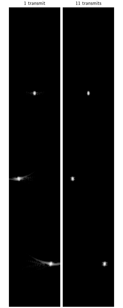
We now restrict the experiment to a single plane wave (normal incidence), by instantiating the operator with the center angle only and beamforming the corresponding transmit. One transmit-receive event per image is what makes ultrafast frame rates possible, at the cost of a point spread function with strong sidelobes and a degraded contrast, shown here against the 11-transmit compounded image.

Tip

You can also create the single-PW physics by updating the existing physics i.e. physics.update(angles=angles[center:center+1]).

center = len(angles) // 2
physics_1pw = dinv.physics.UltrasoundPlaneWave(
    img_size=img_size,
    angles=angles[center : center + 1],
    element_positions=element_positions,
    n_samples=n_samples,
    sampling_frequency=sampling_frequency,
    sound_speed=sound_speed,
    pixel_size=pixel_size,
    pixel_origin=pixel_origin,
    t0=0.0,
    pulse=pulse,
    normalize=False,
    device=device,
    f_number=1.5,
    receive_apod_window="hann",
)
x_1pw = physics_1pw.A_adjoint(y[:, :, center : center + 1])

bmode_1pw = dinv.utils.bmode(x_1pw, dim=-2, amplitude_floor_db=-40, normalize=True)

dinv.utils.plot(
    [bmode_1pw, bmode_das],
    titles=["1 transmit", f"{angles.numel()} transmits"],
    figsize=(4, 10),
)

What next?

Now that you master the basics of ultrafast ultrasound imaging physics, you can go further by

• Reconstructing in-vivo ultrasound images with plug-and-play methods: see the example titled “In-vivo ultrafast ultrasound reconstruction with Plug-and-Play”.

• Simulating your own experiment: probe, medium, acquisition setup, etc.

🏷 Tags: Ultrasound