Reconstruct accelerated non-Cartesian breast MRI acquisition data

This example reconstructs raw non-Cartesian multicoil kspace data from the FastMRI breast dataset [1], for mammography.

The data was acquired using radial sampling, with 288 spokes. We compare image reconstruction using all spokes vs. with 72 spokes (i.e. 4x acceleration). We model the 2D non-uniform FFT physics with deepinv.physics.NonCartesianMRI, which uses MRI-NUFFT.

Note

This example requires the mri-nufft library to model the physics. Install with pip install mri-nufft[finufft] (CPU or MPS) or pip install mri-nufft[cufinufft] (GPU).

You can choose between the various backends, see mri-nufft docs for more details. We suggest using backend='cufinufft' for cuda devices, or backend='finufft' for CPU. For MPS, use backend='mps', which uses finufft but bypasses a torch multithreading problem.

import torch
import deepinv as dinv

device = dinv.utils.get_device()

import importlib

if importlib.util.find_spec("mrinufft") is None:
    raise ImportError(
        "mri-nufft is required for NonCartesianMRI. Install with `pip install mri-nufft[finufft]` (CPU or MPS) or `pip install mri-nufft[cufinufft]` (GPU)."
    )

if torch.device(device).type == "cuda":
    backend = "cufinufft"
elif torch.device(device).type == "mps":
    backend = "mps"
else:
    backend = "finufft"

Selected GPU 0 with 677.25 MiB free memory

Load the non-Cartesian data

The data is originally provided as h5 files, where each file consists of raw kspace for one patient volume, of shape:

• C = channels = 2,

• S = number of spokes = 288,

• Y = number of samples per spoke = 640,

• N = num coils = 16,

• P = partitions = 83 (this will become part of slices = 192)

The data was acquired with a Cartesian fully-sampled partition (slice) readout, and is stored in the frequency domain. Therefore, preprocessing steps are needed to zero-fill the partition axis, then iFFT the partition axis, then take a 2D slice.

For the demo, we perform these steps offline and provide on HuggingFace a sample slice available to download. To reproduce this slice preprocessing, you can run the following code:

import h5py
with h5py.File("/path/to/fastMRI_breast_001_1.h5", "r") as f:
    y = torch.from_numpy(f["kspace"][:, :, :]).float() # C S Y N P

#     y = torch.complex(y[0], y[1]).permute(3, 2, 0, 1) # P N S Y
#     P, N, num_shots, num_samples = y.shape

#     shift = 192 // 2 - 31

#     W = dinv.utils.MRIMixin.ifft(torch.eye(102, dtype=y.dtype), dim=(0,)) # Z,Z centered ifft basis
#     y = torch.einsum("p,pnsy->nsy", W[96, shift : shift + P], y) # Take middle slice -> N S Y
#     y = dinv.utils.MRIMixin.to_torch_complex(y).permute(1, 2, 3, 0) # 2SYN

dinv.utils.download_example(
    "fastMRI_breast_001_1_slice_96.pt", dinv.utils.get_data_home() / "fastMRI_breast"
)

y = torch.load(
    dinv.utils.get_data_home() / "fastMRI_breast" / "fastMRI_breast_001_1_slice_96.pt"
).to(device)

print(
    "Provided slice shape (2, S=num shots, Y=num samples per shot, N=num coils):",
    y.shape,
)

/local/jtachell/deepinv/deepinv/examples/external-libraries/demo_mrinufft_breast.py:74: DeprecationWarning: Function 'get_data_home' is deprecated and will be removed in a future version.
  "fastMRI_breast_001_1_slice_96.pt", dinv.utils.get_data_home() / "fastMRI_breast"
/local/jtachell/deepinv/deepinv/examples/external-libraries/demo_mrinufft_breast.py:78: DeprecationWarning: Function 'get_data_home' is deprecated and will be removed in a future version.
  dinv.utils.get_data_home() / "fastMRI_breast" / "fastMRI_breast_001_1_slice_96.pt"
Provided slice shape (2, S=num shots, Y=num samples per shot, N=num coils): torch.Size([2, 288, 640, 16])

The final kspace should be of shape (1,2,N,S) to be used with deepinv.physics.NonCartesianMRI.

y = y.reshape(2, y.shape[1] * y.shape[2], y.shape[3]).swapaxes(-2, -1).unsqueeze(0)

print("Ready slice shape (1, 2, N, S*Y):", y.shape)

Ready slice shape (1, 2, N, S*Y): torch.Size([1, 2, 16, 184320])

Fully-sampled reconstruction

We compute the root-sum-squares reconstruction with all 288 angles, bypassing the need to estimate coil maps. This reconstruction consists of the adjoint of density compensated kspace, and can be seen as an approximate pseudo-inverse.

The FastMRI data was acquired with golden-angle radial sampling, with 640 samples per shot, and sampling from center outwards. We use the standard reconstruction size of 320*320.

physics_fs = dinv.physics.NonCartesianMRI(
    img_size=(320, 320),
    num_shots=288,
    num_samples_per_shot=640,
    coil_maps=y.shape[2],  # = 16 to construct physics correctly. Not used for RSS
    trajectory="radial",
    tilt="golden",
    in_out=True,
    backend=backend,
    device=device,
    normalize=True,
)

with torch.no_grad():
    x = physics_fs.A_dagger(y, density_compensate=True, rss=True)  # 1, H, W

/local/jtachell/deepinv/deepinv/.pixi/envs/docs/lib/python3.12/site-packages/mrinufft/_utils.py:67: UserWarning: Samples will be rescaled to [-pi, pi), assuming they were in [-0.5, 0.5)
  warnings.warn(
Power iteration converged at iteration 12, ||A^T A||_2=117.25

Reconstruct accelerated data

We undersample the radial data by taking the first few (golden angle) shots. We construct the accelerated non-Cartesian MRI physics, and we empirically normalise the physics for solvers that require this. Then, we estimate the coil sensitivity maps using ESPIRiT (on a lower dimensional image).

undersampling_factor = 4

y = y[..., : y.shape[-1] // undersampling_factor]

physics = dinv.physics.NonCartesianMRI(
    img_size=(320, 320),
    num_shots=288 // undersampling_factor,
    num_samples_per_shot=640,
    coil_maps=y.shape[2],  # dummy. Update with real maps below
    trajectory="radial",
    tilt="golden",
    in_out=True,
    backend=backend,
    device=device,
    normalize=True,
    noise_model=dinv.physics.GaussianNoise(0.001),
)

coil_maps = physics.estimate_coil_maps(y, method="espirit", decim=4)
physics.update(coil_maps=coil_maps)

Power iteration converged at iteration 9, ||A^T A||_2=29.31

  0%|          | 0/10 [00:00<?, ?it/s]
 10%|█         | 1/10 [00:00<00:01,  5.46it/s]
 20%|██        | 2/10 [00:00<00:01,  5.48it/s]
 30%|███       | 3/10 [00:00<00:01,  5.49it/s]
 40%|████      | 4/10 [00:00<00:01,  5.50it/s]
 50%|█████     | 5/10 [00:00<00:00,  5.49it/s]
 60%|██████    | 6/10 [00:01<00:00,  5.48it/s]
 70%|███████   | 7/10 [00:01<00:00,  5.48it/s]
 80%|████████  | 8/10 [00:01<00:00,  5.49it/s]
 90%|█████████ | 9/10 [00:01<00:00,  5.50it/s]
100%|██████████| 10/10 [00:01<00:00,  5.49it/s]
100%|██████████| 10/10 [00:01<00:00,  5.49it/s]
/local/jtachell/deepinv/deepinv/.pixi/envs/docs/lib/python3.12/site-packages/mrinufft/operators/base.py:1075: UserWarning: Lipschitz constant did not converge
  warnings.warn("Lipschitz constant did not converge")

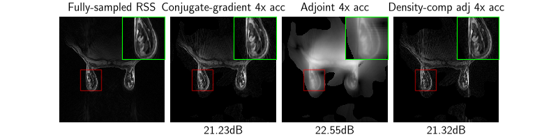
Reconstruct with conjugate-gradient

We reconstruct the data with the conjugate-gradient (CG) algorithm, which gives a least-squares solution. Notice that streak artifacts are present, which are expected for CG on undersampled data. We compare also to the adjoint (which should be overwhelmingly low-freq) and the density-compensated adjoint (which gives a fast approximation to the least-squares solution by pre-filtering y).

with torch.no_grad():
    x_cg = physics.A_dagger(y)
    x_adj = physics.A_adjoint(y)
    x_dc = physics.A_dagger(y, density_compensate=True)

# Magnitude images for computing metrics
x_cg = dinv.utils.complex_abs(x_cg)
x_adj = dinv.utils.complex_abs(x_adj)
x_dc = dinv.utils.complex_abs(x_dc)

metric = dinv.metric.PSNR(max_pixel=None, min_pixel=None)

dinv.utils.plot(
    [x, x_cg, x_adj, x_dc],
    titles=[
        "Fully-sampled RSS",
        "Conjugate-gradient 4x acc",
        "Adjoint 4x acc",
        "Density-comp adj 4x acc",
    ],
    subtitles=[
        "",
        f"{metric(x_cg, x).item():.2f}dB",
        f"{metric(x_adj, x).item():.2f}dB",
        f"{metric(x_dc, x).item():.2f}dB",
    ],
    plot_inset=True,
    extract_loc=(0.2, 0.5),
    inset_loc=(0.6, 0),
)

What’s next?

We didn’t show any model-based on deep learning reconstruction methods in this example to keep the example lightweight. You can try out other types of reconstruction algorithms listed in the user guide.

Interested in non-Cartesian MRI? You can dive deeper into mri-nufft, which has extensive features such as more advanced trajectories, trajectory estimation, various coil map estimation algorithms or off-resonance correction.

References:

[1]

Eddy Solomon, Patricia Johnson, Zhengguo Tan, Radhika Tibrewala, Yvonne Lui, Florian Knoll, Linda Moy, Sungheon Gene Kim, and Laura Heacock. Fastmri breast: a publicly available radial k-space dataset of breast dynamic contrast-enhanced mri. Radiology Artificial Intelligence, 2025. doi:10.1148/ryai.240345.