Noisy data-fidelity terms for diffusion posterior sampling

This example compares six approximations of the measurement-matching term used by diffusion posterior samplers.

Three of them measure the mismatch directly at the noisy iterate \(x_t\), and therefore need no denoiser evaluation at all:

• Score-based Annealed Langevin Dynamics (Score-ALD) Jalal et al.[1],

• Score-SDE Song et al.[2],

• Iterative Latent Variable Refinement (ILVR) Choi et al.[3].

The other three first denoise \(x_t\), and differ in how much of the conditional uncertainty they keep:

• Diffusion Posterior Sampling (DPS) Chung et al.[4],

• Pseudoinverse-Guided Diffusion Models (PiGDM) Song et al.[5],

• Moment Matching Rozet et al.[6].

We follow the presentation of A Survey on Diffusion Models for Inverse Problems Daras et al.[7], which reviews these and other ways of incorporating measurements into diffusion models.

Here, we focus on the noisy data-fidelity term itself. For a complete DPS reconstruction, including the diffusion schedule and reverse-time sampling loop, see DPS – Posterior Sampling with Diffusion Models. For a tutorial on assembling a posterior sampler from an SDE, a solver, and a data-fidelity term, see Building your diffusion posterior sampling method using SDEs.

Posterior sampling and the intractable likelihood

We use a Variance-Exploding (VE) diffusion, whose scaling is \(s(t)=1\):

\[x_t = x_0 + \sigma_t\omega, \qquad \omega\sim\mathcal N(0,\mathrm I).\]

By Bayes’ rule, the conditional score is

\[\nabla_{x_t}\log p_t(x_t\mid y) = \nabla_{x_t}\log p_t(x_t) + \nabla_{x_t}\log p_t(y\mid x_t).\]

A diffusion denoiser \(D_\sigma\) estimates the unconditional part using Tweedie’s formula. The second term is harder because

\[p_t(y\mid x_t) = \int p(y\mid x_0)p(x_0\mid x_t)\,\mathrm d x_0\]

is generally intractable. The goal of the methods below is to replace \(p(x_0\mid x_t)\) by a Gaussian approximation

\[p(x_0\mid x_t) \approx \mathcal N\!\left( x_0;D_{\sigma_t}(x_t),\Sigma_t(x_t) \right).\]

For a linear forward model and Gaussian measurement noise, the integral of the two Gaussian densities is available in closed form:

\[p_t(y\mid x_t) \approx \mathcal N\!\left( y;A D_{\sigma_t}(x_t), A\Sigma_t(x_t) A^\top + \mathrm I \right).\]

The approximations differ primarily in their choice of \(\Sigma_t(x_t)\). DPS is the degenerate, zero-covariance case; PiGDM uses an isotropic covariance; and Moment Matching estimates a structured covariance with the second-order Tweedie formula. A deepinv.sampling.NoisyDataFidelity approximates the gradient of the resulting negative log-likelihood. Consequently, deepinv.sampling.PosteriorDiffusion subtracts the gradient returned by the data-fidelity object from the unconditional score.

The word noisy here refers to the diffusion-corrupted variable \(x_t\); the measurements themselves do not have to be noisy.

Create one inverse problem and one noisy diffusion state

We use linear inpainting here. DPS also supports differentiable nonlinear forward operators, whereas the PiGDM and Moment Matching implementations below require a linear operator.

import matplotlib.pyplot as plt
import torch

import deepinv as dinv

device = dinv.utils.get_device()
dtype = torch.float32 if "mps" in str(device) else torch.float64

x_true = dinv.utils.load_example(
    "FFHQ_example.png", img_size=64, resize_mode="resize", device=device
)
mask = torch.ones_like(x_true)
mask[..., 24:40, 24:40] = 0.0
measurement_noise = 0.05
physics = dinv.physics.Inpainting(
    img_size=x_true.shape[1:],
    mask=mask,
    device=device,
    noise_model=dinv.physics.GaussianNoise(sigma=measurement_noise),
)
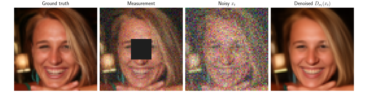
y = physics(x_true)

sigma_t = 0.15
rng = torch.Generator(device=device).manual_seed(0)
x_t = x_true + sigma_t * torch.randn(
    x_true.shape, generator=rng, device=device, dtype=x_true.dtype
)

# We use the same FFHQ NCSNpp denoiser for every approximation.
denoiser = dinv.models.NCSNpp(pretrained="download").to(device)
with torch.no_grad():
    x_0_denoised = denoiser(x_t, sigma_t)

dinv.utils.plot(
    {
        "Ground truth": x_true,
        "Measurement": y,
        r"Noisy $x_t$": x_t,
        r"Denoised $D_{\sigma_t}(x_t)$": x_0_denoised,
    },
    figsize=(12, 3),
)

Selected GPU 0 with 18109.5625 MiB free memory

Score-ALD: guide with the noisy iterate itself

The cheapest option is not to denoise at all. Score-ALD Jalal et al.[1] evaluates the measurement mismatch directly at \(x_t\), and compensates for the fact that \(x_t\) is noisy by inflating the measurement noise variance with an annealing parameter \(\gamma_t\):

\[p_t(y\mid x_t) \approx \mathcal N\!\left( y; A x_t, (\sigma_y^2+\gamma_t^2)\mathrm I \right),\]

which gives the guidance

\[\nabla_{x_t}\log p_t(x_t\mid y) \approx \nabla_{x_t}\log p_t(x_t) - \lambda \frac{A^\top (A x_t - y)}{\sigma_y^2+\gamma_t^2}.\]

By default \(\gamma_t=\sigma_t\), so the guidance is weak early in the diffusion, when \(x_t\) is mostly noise, and strengthens as \(\sigma_t\to 0\). Because that denominator already sets the scale, weight=1 is the natural choice here.

ald = dinv.sampling.ALDDataFidelity(weight=1.0)

Score-SDE and ILVR: noise the measurements instead

Score-SDE Song et al.[2] makes the same comparison, but first lifts the measurements to the current noise level,

\[y_t = y + \sigma_t\epsilon, \qquad \epsilon\sim\mathcal N(0,\mathrm I),\]

so that \(y_t\) and \(A x_t\) are corrupted by comparable amounts of noise. ILVR Choi et al.[3] differs only in how the measurement residual is lifted back to the image space: it uses the pseudo-inverse \(A^\dagger\) rather than the adjoint \(A^\top\),

\[\nabla_{x_t}\log p_t(x_t\mid y) \approx \nabla_{x_t}\log p_t(x_t) - \lambda \frac{A^\dagger (A x_t - y_t)}{\sigma_y^2+\gamma_t^2}.\]

score_sde = dinv.sampling.ScoreSDEDataFidelity(weight=1.0)
ilvr = dinv.sampling.ILVRDataFidelity(weight=1.0)

DPS: plug in the denoised posterior mean

DPS Chung et al.[4] approximates the conditional distribution by a Dirac mass at the denoised posterior mean:

\[p(x_0\mid x_t) \approx \delta\!\left( x_0-D_{\sigma_t}(x_t) \right), \qquad D_{\sigma_t}(x_t) \simeq \mathbb E[x_0\mid x_t].\]

This is the degenerate Gaussian approximation \(\Sigma_t(x_t)=0\). Inserting it into the integral gives \(p_t(y\mid x_t)\approx p(y\mid D_{\sigma_t}(x_t))\). Note that this is equivalent to differentiating the residual norm:

\[\nabla_{x_t}\log p_t(x_t\mid y) \approx \nabla_{x_t}\log p_t(x_t) - \lambda\nabla_{x_t} \left\|A D_{\sigma_t}(x_t)-y\right\|_2.\]

In deepinv.sampling.DPSDataFidelity, \(\lambda\) is the weight parameter. It controls the scale of the data-fidelity contribution relative to the unconditional prior score: a larger value enforces the measurements more strongly.

The residual norm above carries no noise variance, so \(\lambda\) has to absorb a factor of order \(\|A D_{\sigma_t}(x_t)-y\|/\sigma_y^2\), in the hundreds here. To keep weight on the same scale as the other terms, we use guidance="annealed", which differentiates the Gaussian negative log-likelihood with the annealed variance \(\sigma_y^2+\sigma_t^2\) instead:

\[\nabla_{x_t}\log p_t(x_t\mid y) \approx \nabla_{x_t}\log p_t(x_t) - \lambda\nabla_{x_t} \frac{\left\|A D_{\sigma_t}(x_t)-y\right\|_2^2}{2(\sigma_y^2+\sigma_t^2)}.\]

Pass guidance="norm" (the default) for the residual norm of the original paper.

dps = dinv.sampling.DPSDataFidelity(denoiser=denoiser, weight=1.0, guidance="annealed")

PiGDM: use an isotropic covariance approximation

PiGDM Song et al.[5] retains conditional uncertainty but approximates it with an isotropic Gaussian:

\[p(x_0\mid x_t) \approx \mathcal N\!\left( x_0;D_{\sigma_t}(x_t),\Sigma_t(x_t) \right), \qquad \Sigma_t(x_t)=r_t^2\mathrm I, \qquad r_t^2=\frac{\sigma_t^2}{1+\sigma_t^2}.\]

Writing \(J_D\) for the denoiser Jacobian, the resulting gradient is

\[\nabla_{x_t}\log p_t(x_t\mid y) \approx \nabla_{x_t}\log p_t(x_t) - \lambda J_D^\top A^\top (r_t^2 A A^\top + \sigma_y^2\mathrm I)^{-1} (A D_{\sigma_t}(x_t)-y),\]

where \(\sigma_y\) is the standard deviation of the measurement noise, read from physics.noise_model.sigma.

The inverse is evaluated exactly for deepinv.physics.DecomposablePhysics operators and with conjugate gradient for other linear operators. Jacobian-vector products are computed automatically, without forming \(J_D\) explicitly. The \(\lambda\) factor is exposed as weight in deepinv.sampling.PiGDMDataFidelity; increasing it strengthens the data-fidelity contribution relative to the unconditional prior score.

pigdm_weight = 1
pigdm = dinv.sampling.PiGDMDataFidelity(
    denoiser=denoiser,
    weight=pigdm_weight,
    cg_max_iter=10,
)

Moment Matching: retain a structured covariance

Moment Matching Rozet et al.[6] uses the denoiser Jacobian to approximate the conditional covariance rather than replacing it by an isotropic scalar. In our additive Gaussian parametrization, the second-order Tweedie formulas give

\[\Sigma_t(x_t) = \operatorname{Cov}[x_0\mid x_t] = \sigma_t^2 J_D(x_t,\sigma_t)\]

Moment Matching explicitly approximates the conditional distribution by the anisotropic Gaussian with this covariance:

\[p(x_0\mid x_t) \approx \mathcal N\!\left( x_0;D_{\sigma_t}(x_t),\Sigma_t(x_t) \right).\]

The resulting gradient is

\[\nabla_{x_t}\log p_t(x_t\mid y) \approx \nabla_{x_t}\log p_t(x_t) - \lambda J_D^\top A^\top (\sigma_t^2 A J_D A^\top + \sigma_y^2\mathrm I)^{-1} (A D_{\sigma_t}(x_t)-y).\]

This can capture direction-dependent uncertainty, at the cost of solving a denoiser-dependent linear system. DeepInverse evaluates the system with conjugate gradient and uses vector-Jacobian products throughout. The \(\lambda\) factor is the weight parameter of deepinv.sampling.MomentMatchingDataFidelity; increasing it gives the data-fidelity contribution more influence relative to the unconditional prior score.

moment_matching_weight = 1
moment_matching = dinv.sampling.MomentMatchingDataFidelity(
    denoiser=denoiser,
    weight=moment_matching_weight,
    cg_max_iter=3,
)

Compare the guidance terms

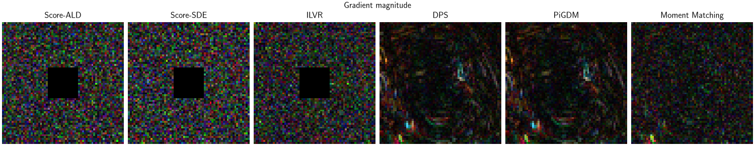
Calling grad is enough to compare the six approximations at the same \(x_t\). Their scales are method-dependent, so weight should be tuned separately in a reconstruction. The plot independently normalizes the magnitude of each gradient to emphasize its spatial structure.

The two families look different:

Score-ALD, Score-SDE and ILVR compare the noisy iterate to the measurements. Here \(x_t = x_0 + \sigma_t\omega\) is built from the ground truth, so

\[A x_t - y = A(x_0 + \sigma_t\omega) - (A x_0 + \sigma_y\eta) = \sigma_t A\omega - \sigma_y\eta :\]

the signal cancels exactly, and the residual is pure noise. Their guidance maps therefore look like noise, and they vanish on the masked pixels, where \(A^\top\) and \(A^\dagger\) are zero.

DPS, PiGDM and Moment Matching instead compare a denoised estimate to the measurements, so their residual reflects genuine reconstruction error rather than the noise in \(x_t\). Backpropagating it through the denoiser spreads the guidance over the whole image, including inside the mask.

data_fidelities = {
    "Score-ALD": ald,
    "Score-SDE": score_sde,
    "ILVR": ilvr,
    "DPS": dps,
    "PiGDM": pigdm,
    "Moment Matching": moment_matching,
}

gradients = {}
for name, data_fidelity in data_fidelities.items():
    gradient = data_fidelity.grad(x_t.clone(), y=y, physics=physics, sigma=sigma_t)
    gradients[name] = gradient
    norm = torch.linalg.vector_norm(gradient).item()
    print(f"{name:>15s} gradient norm: {norm:.3e}")

dinv.utils.plot(
    {f"{name}": gradient.abs() for name, gradient in gradients.items()},
    figsize=(15, 3),
    suptitle="Gradient magnitude",
)

      Score-ALD gradient norm: 4.287e+02
      Score-SDE gradient norm: 7.782e+02
           ILVR gradient norm: 7.708e+02
            DPS gradient norm: 1.146e+02
          PiGDM gradient norm: 1.169e+02
Moment Matching gradient norm: 1.978e+02

Posterior sampling experiment

The noisy data-fidelity object is one interchangeable component of deepinv.sampling.PosteriorDiffusion. We now hold the denoiser, VE diffusion, Euler solver, measurements, and random seed fixed, and change only the noisy data-fidelity approximation. Using the same seed gives every method the same initial noise and Brownian increments.

All six use weight=1: every term is normalized by a guidance strength of order \(\sigma_y^2+\sigma_t^2\), so a single scale works for all of them.

Moment Matching is considerably slower on CPU because every diffusion step contains an inner conjugate-gradient solve. On CPU, we therefore display a precomputed reconstruction; on GPU and MPS devices, we compute it normally.

num_steps = 100
timesteps = torch.linspace(
    1.0,
    0.001,
    num_steps,
    device=device,
    dtype=dtype,
)

sde = dinv.sampling.VarianceExplodingDiffusion(
    alpha=0.25,
    device=device,
    dtype=dtype,
)

posterior_samples = {}
for name, data_fidelity in data_fidelities.items():
    if name == "Moment Matching" and device.type == "cpu":
        precomputed_sample = dinv.utils.load_url_image(
            "https://huggingface.co/deepinv/demo/resolve/main/" "moment_matching.png",
            device=device,
            dtype=x_true.dtype,
        )
        posterior_samples[name] = precomputed_sample[:, : x_true.shape[1]]
        continue

    solver = dinv.sampling.EulerSolver(
        timesteps=timesteps,
        rng=torch.Generator(device=device),
    )
    posterior_sampler = dinv.sampling.PosteriorDiffusion(
        data_fidelity=data_fidelity,
        denoiser=denoiser,
        sde=sde,
        solver=solver,
        device=device,
        dtype=dtype,
        verbose=False,
    )

    with torch.no_grad():
        posterior_samples[name] = posterior_sampler(
            y=y,
            physics=physics,
            seed=1,
            denoise_output=True,
        ).clip(0.0, 1.0)

# One row per family: the denoiser-free terms on top, the denoiser-based ones
# below, each preceded by its reference image.
rows = [
    {
        "Ground truth": x_true,
        **{
            name: posterior_samples[name] for name in ("Score-ALD", "Score-SDE", "ILVR")
        },
    },
    {
        "Measurement": y,
        **{
            name: posterior_samples[name]
            for name in ("DPS", "PiGDM", "Moment Matching")
        },
    },
]

fig, axs = plt.subplots(
    len(rows), 4, figsize=(12, 6.5), squeeze=False, layout="compressed"
)
for row, images in zip(axs, rows, strict=True):
    dinv.utils.plot(images, fig=fig, axs=row[None, :], show=False)
plt.show()

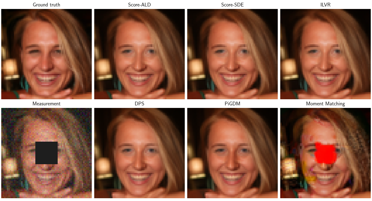
All six recover the masked region, at very different costs: Score-ALD, Score-SDE and ILVR need no denoiser evaluation for the guidance term, DPS needs one backward pass through the denoiser, and PiGDM and Moment Matching need a linear solve on top.

References:

[1] (1,2)

Ajil Jalal, Marius Arvinte, Giannis Daras, Eric Price, Alexandros G Dimakis, and Jon Tamir. Robust compressed sensing mri with deep generative priors. Advances in Neural Information Processing Systems, 34:14938–14954, 2021.

[2] (1,2)

Yang Song, Jascha Sohl-Dickstein, Diederik P Kingma, Abhishek Kumar, Stefano Ermon, and Ben Poole. Score-based generative modeling through stochastic differential equations. In International Conference on Learning Representations. 2020.

[3] (1,2)

Jooyoung Choi, Sungwon Kim, Yonghyun Jeong, Youngjune Gwon, and Sungroh Yoon. Ilvr: conditioning method for denoising diffusion probabilistic models. In 2021 IEEE/CVF International Conference on Computer Vision (ICCV), 14347–14356. IEEE, 2021.

[4] (1,2)

Hyungjin Chung, Jeongsol Kim, Michael Thompson Mccann, Marc Louis Klasky, and Jong Chul Ye. Diffusion posterior sampling for general noisy inverse problems. In The Eleventh International Conference on Learning Representations. 2022.

[5] (1,2)

Jiaming Song, Arash Vahdat, Morteza Mardani, and Jan Kautz. Pseudoinverse-guided diffusion models for inverse problems. In International conference on learning representations. 2023.

[6] (1,2)

François Rozet, Gérôme Andry, François Lanusse, and Gilles Louppe. Learning diffusion priors from observations by expectation maximization. Advances in Neural Information Processing Systems, 37:87647–87682, 2024.

[7]

Giannis Daras, Hyungjin Chung, Chieh-Hsin Lai, Yuki Mitsufuji, Jong Chul Ye, Peyman Milanfar, Alexandros G. Dimakis, and Mauricio Delbracio. A survey on diffusion models for inverse problems. arXiv preprint arXiv:2410.00083, 2024.