OSEM, BSREM and gradient descent for 2D BrainWeb PET

This example reconstructs a 2D slice from the BrainWeb casperdcl/brainweb positron emission tomography (PET) dataset. The slice contains five hot lesions, we simulate a sinogram with deepinv.physics.PET and we compare standard PET reconstruction algorithms with methods that support penalized objective functions.

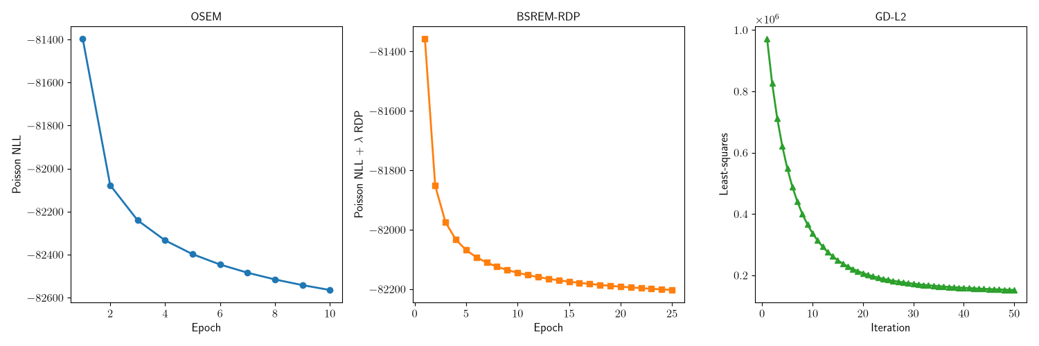
OSEM and BSREM minimize the Poisson negative log-likelihood

\[f(x) = \mathbf{1}^T(Ax+b) - y^T\log(Ax+b),\]

and BSREM additionally uses the Relative Difference Prior (RDP) deepinv.optim.RDP as \(\regname\) in \(f(x)+\lambda\reg{x}\). RDP favors sharp transitions in reconstructed images, and adapts to the local signal level, which is particularly useful for emission tomography where the dynamic can be large. We also demonstrate general-purpose gradient descent with a least-squares objective.

Note

This example requires the brainweb and parallelproj packages. Install with pip install brainweb parallelproj.

import matplotlib.pyplot as plt
import parallelproj
import torch
from array_api_compat import torch as torch_compat
from torch.utils.data import DataLoader

import deepinv as dinv
from deepinv.datasets import BrainWebPET
from deepinv.physics import PET

Load a BrainWeb slice

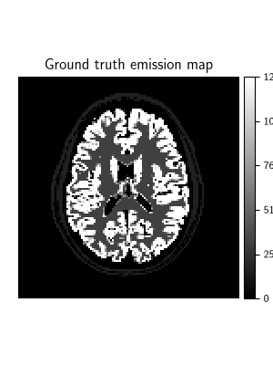
We begin by loading a volume through deepinv.datasets.BrainWebPET, which follows the (C, D, H, W) convention. We select its middle axial slice and center-crop it in the transverse plane. The data loader adds the leading batch dimension expected by the physics and reconstruction code.

device = torch.device("cuda" if torch.cuda.is_available() else "cpu")
image_size = (120, 120)


def center_slice_2d(volume):
    middle_d = volume.shape[-3] // 2
    crop_slices = tuple(
        slice((size - crop) // 2, (size + crop) // 2)
        for size, crop in zip(volume.shape[-2:], image_size, strict=True)
    )
    return volume[(..., middle_d, *crop_slices)]


dataset = BrainWebPET(subject_ids=4, transform=center_slice_2d, use_dict_output=True)
dataloader = DataLoader(dataset, batch_size=1, shuffle=False)
batch = next(iter(dataloader))
x = batch["x"].to(device)

dinv.utils.plot(x, titles="Ground truth emission map", cbar=True, figsize=(3, 4))

/local/jtachell/deepinv/deepinv/.pixi/envs/docs/lib/python3.12/site-packages/brainweb/utils.py:13: DeprecationWarning: Please import `gaussian_filter` from the `scipy.ndimage` namespace; the `scipy.ndimage.filters` namespace is deprecated and will be removed in SciPy 2.0.0.
  from scipy.ndimage.filters import gaussian_filter
/local/jtachell/deepinv/deepinv/deepinv/utils/plotting.py:493: UserWarning: set_ticklabels() should only be used with a fixed number of ticks, i.e. after set_ticks() or using a FixedLocator. Otherwise, ticks may be mislabeled.
  colbar.set_ticklabels(true_labels)
/local/jtachell/deepinv/deepinv/deepinv/utils/plotting.py:513: UserWarning: This figure was using a layout engine that is incompatible with subplots_adjust and/or tight_layout; not calling subplots_adjust.
  plt.subplots_adjust(hspace=0.2, wspace=0.2)

Add hot lesions

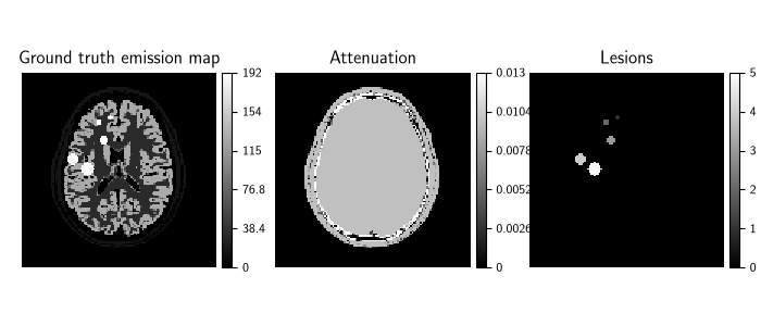
Although the original BrainWeb volumes contain no lesions, deepinv.datasets.BrainWebPET can add synthetic lesions with configurable properties such as size and intensity. Here, we add five lesions with increasing diameters and equal intensity. With the fixed seed, all five lesions intersect the selected middle slice.

lesion_diameters = [5, 8, 11, 14, 17]  # mm
lesion_dataset = BrainWebPET(
    subject_ids=4,
    transform=center_slice_2d,
    lesion_diameters=lesion_diameters,
    lesion_kwargs={
        "intensity": [192.0] * len(lesion_diameters),
        "blur": [0.0] * len(lesion_diameters),
        "thresh": 30,
    },
    seed=0,
    use_dict_output=True,
)
lesion_dataloader = DataLoader(lesion_dataset, batch_size=1, shuffle=False)
batch = next(iter(lesion_dataloader))
x = batch["x"].to(device)
attenuation = batch["params"]["attenuation"].to(device)
lesion_mask = batch["params"]["lesion_mask"].to(device)

dinv.utils.plot(
    [x, attenuation, lesion_mask],
    titles=["Ground truth emission map", "Attenuation", "Lesions"],
    cbar=True,
    figsize=(7, 3),
)

/local/jtachell/deepinv/deepinv/deepinv/utils/plotting.py:493: UserWarning: set_ticklabels() should only be used with a fixed number of ticks, i.e. after set_ticks() or using a FixedLocator. Otherwise, ticks may be mislabeled.
  colbar.set_ticklabels(true_labels)
/local/jtachell/deepinv/deepinv/deepinv/utils/plotting.py:493: UserWarning: set_ticklabels() should only be used with a fixed number of ticks, i.e. after set_ticks() or using a FixedLocator. Otherwise, ticks may be mislabeled.
  colbar.set_ticklabels(true_labels)
/local/jtachell/deepinv/deepinv/deepinv/utils/plotting.py:493: UserWarning: set_ticklabels() should only be used with a fixed number of ticks, i.e. after set_ticks() or using a FixedLocator. Otherwise, ticks may be mislabeled.
  colbar.set_ticklabels(true_labels)
/local/jtachell/deepinv/deepinv/deepinv/utils/plotting.py:513: UserWarning: This figure was using a layout engine that is incompatible with subplots_adjust and/or tight_layout; not calling subplots_adjust.
  plt.subplots_adjust(hspace=0.2, wspace=0.2)

Define scanner geometry and construct PET physics

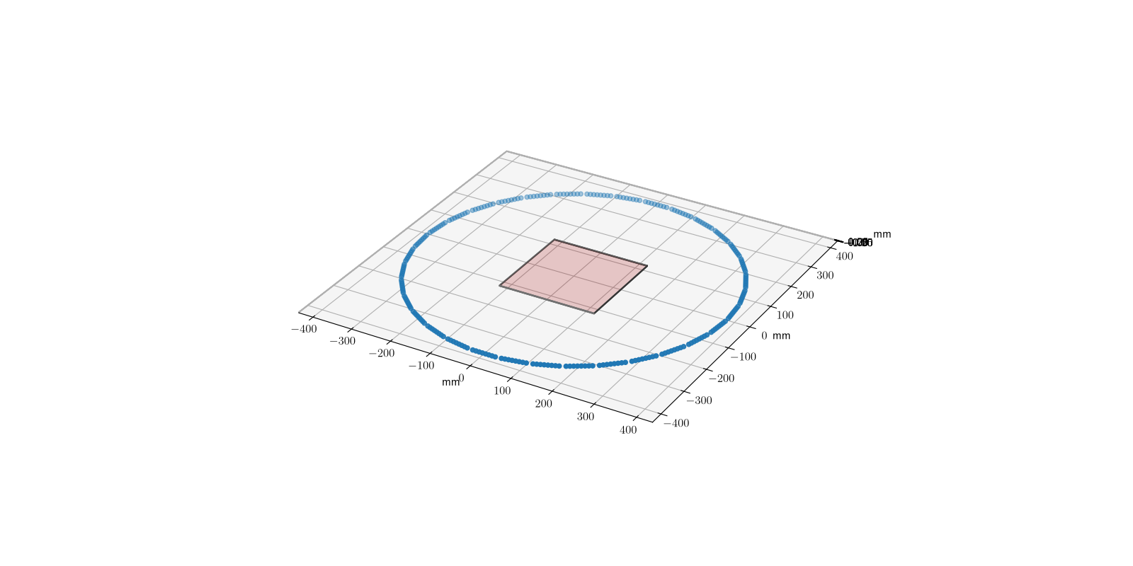
A single detector ring defines the 2D acquisition. As in the 3D example, we halve the number of detector endpoints per polygon side and double their spacing, approximately preserving the transaxial field of view at a lower sampling resolution.

scanner = parallelproj.pet_scanners.DemoPETScannerGeometry(
    torch_compat,
    dev=device,
    num_rings=1,
    num_sides=34,
    num_lor_endpoints_per_side=8,
    lor_spacing=8,
)
physics = PET(
    img_size=x.shape[2:],
    voxel_size=(2, 2),
    scanner=scanner,
    attenuation=attenuation,
    fwhm_data_mm=3.0,
    gain=1.0,
    normalize=True,
    normalize_counts=True,
    device=device,
)

physics.plot_geometry()

Acquisition simulation

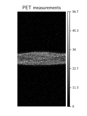
# We simulate a relatively low-count acquisition with approximately 50,000 counts.
# A spatially uniform background provides a simple approximation of random and scattered coincidences.
# Its expected event count is 20% of the expected true coincidence count.

# .. tip:
#
#   Alternatively, instead of simulating the acquisition, we could load real sinogram data matching this acquisition geometry here.


expected_signal = physics.A(x)
target_prompt_counts = 5e4
background_to_signal_ratio = 0.2
background = torch.full_like(
    expected_signal,
    background_to_signal_ratio * expected_signal.mean(),
)
gain = (expected_signal.sum() + background.sum()).item() / target_prompt_counts
physics.noise_model.update_parameters(gain=gain)

# The sinogram is drawn once from the combined signal and background rate.
physics.update(background=background)
torch.manual_seed(0)

y = physics(x)

realized_prompt_counts = round((y / gain).sum().item())
print(
    f"Expected prompt counts: {target_prompt_counts:,}; "
    f"realized: {realized_prompt_counts:,}; "
    f"background fraction: "
    f"{background_to_signal_ratio / (1 + background_to_signal_ratio):.1%}"
)

dinv.utils.plot([y], ["PET measurements"], figsize=(3, 4), cbar=True)

Expected prompt counts: 50,000.0; realized: 50,302; background fraction: 16.7%
/local/jtachell/deepinv/deepinv/deepinv/utils/plotting.py:493: UserWarning: set_ticklabels() should only be used with a fixed number of ticks, i.e. after set_ticks() or using a FixedLocator. Otherwise, ticks may be mislabeled.
  colbar.set_ticklabels(true_labels)
/local/jtachell/deepinv/deepinv/deepinv/utils/plotting.py:513: UserWarning: This figure was using a layout engine that is incompatible with subplots_adjust and/or tight_layout; not calling subplots_adjust.
  plt.subplots_adjust(hspace=0.2, wspace=0.2)

Configure objectives and per-iteration metrics

PET reconstruction commonly minimizes the Poisson negative log-likelihood. We regularize this objective with the Relative Difference Prior (RDP) introduced by Nuyts et al.[1]; see deepinv.optim.RDP for implementation details. For a nonnegative image \(x\), the RDP is

\[\operatorname{RDP}_{\gamma}(x) = \sum_{\{j,k\}\in\mathcal{N}} \frac{(x_j-x_k)^2}{x_j+x_k+\gamma|x_j-x_k|},\]

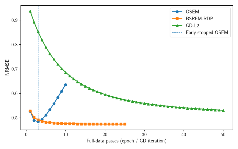
where \(\mathcal{N}\) contains each pair of neighboring pixels once, and \(\gamma\) controls edge preservation. We monitor reconstruction quality at each iteration using the normalized root mean squared error (NRMSE).

data_fidelity = dinv.optim.PoissonLikelihood(
    gain=gain,
    bkg=background / gain,
    denormalize=True,
)
rdp = dinv.optim.RDP(gamma=4.0)
lambda_reg = 0.008
nrmse = dinv.metric.NRMSE()


def reconstruction_nrmse(metric_history, x_prev, x_cur):
    return nrmse(x_cur.unsqueeze(0), x).item()


def poisson_nll(metric_history, x_prev, x_cur):
    return data_fidelity(x_cur.unsqueeze(0), y, physics).item()


def penalized_poisson_nll(metric_history, x_prev, x_cur):
    x_cur = x_cur.unsqueeze(0)
    return (data_fidelity(x_cur, y, physics) + lambda_reg * rdp(x_cur)).item()


metrics = {
    "nrmse": reconstruction_nrmse,
    "poisson_nll": poisson_nll,
    "penalized_poisson_nll": penalized_poisson_nll,
}

Reconstruct with OSEM and BSREM-RDP

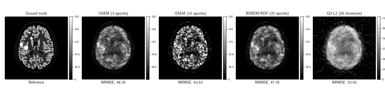
Ordered Subsets Expectation Maximization (OSEM) [2] is an accelerated form of MLEM [3] and a standard baseline for PET reconstruction. At low counts, however, later OSEM iterates increasingly amplify noise, so the algorithm is often stopped early. Because the ground truth is available in this simulation, we can select a suitable stopping point using the reconstruction error. In practice, the stopping point must be chosen without a reference image and may vary between acquisitions.

Block-Sequential Regularized Expectation Maximization (BSREM) [4] incorporates a regularization term to suppress noise while retaining convergence guarantees. We use the RDP and stop BSREM after 25 epochs.

num_subsets = 4
osem_early_iter = 3
num_iter_osem = 10
num_epochs_bsrem = 25
initialization = torch.ones_like(x)
initial_relaxation = 1
relaxation_decay = 0.8
stepsize = [
    initial_relaxation / (1.0 + relaxation_decay * k) for k in range(num_epochs_bsrem)
]

osem_early = dinv.optim.OSEM(
    data_fidelity=data_fidelity,
    num_subsets=num_subsets,
    max_iter=osem_early_iter,
)
osem = dinv.optim.OSEM(
    data_fidelity=data_fidelity,
    num_subsets=num_subsets,
    max_iter=num_iter_osem,
    custom_metrics=metrics,
    verbose=True,
    show_progress_bar=True,
)
bsrem = dinv.optim.BSREM(
    data_fidelity=data_fidelity,
    prior=rdp,
    lambda_reg=lambda_reg,
    num_subsets=num_subsets,
    stepsize=stepsize,
    max_iter=num_epochs_bsrem,
    custom_metrics=metrics,
    verbose=True,
    show_progress_bar=True,
)

x_osem_early = osem_early(y, physics, init=initialization)
x_osem, metrics_osem = osem(y, physics, init=initialization, compute_metrics=True)
x_bsrem, metrics_bsrem = bsrem(y, physics, init=initialization, compute_metrics=True)

  0%|          | 0/10 [00:00<?, ?it/s]
 30%|███       | 3/10 [00:00<00:00, 20.27it/s]
 60%|██████    | 6/10 [00:00<00:00, 20.26it/s]
 90%|█████████ | 9/10 [00:00<00:00, 20.25it/s]
100%|██████████| 10/10 [00:00<00:00, 20.23it/s]

  0%|          | 0/25 [00:00<?, ?it/s]
  8%|▊         | 2/25 [00:00<00:01, 16.86it/s]
 16%|█▌        | 4/25 [00:00<00:01, 16.88it/s]
 24%|██▍       | 6/25 [00:00<00:01, 16.89it/s]
 32%|███▏      | 8/25 [00:00<00:01, 16.89it/s]
 40%|████      | 10/25 [00:00<00:00, 16.89it/s]
 48%|████▊     | 12/25 [00:00<00:00, 16.90it/s]
 56%|█████▌    | 14/25 [00:00<00:00, 16.91it/s]
 64%|██████▍   | 16/25 [00:00<00:00, 16.92it/s]
 72%|███████▏  | 18/25 [00:01<00:00, 16.91it/s]
 80%|████████  | 20/25 [00:01<00:00, 16.92it/s]
 88%|████████▊ | 22/25 [00:01<00:00, 16.93it/s]
 96%|█████████▌| 24/25 [00:01<00:00, 16.93it/s]
100%|██████████| 25/25 [00:01<00:00, 16.91it/s]

Reconstruct with gradient descent and an L2 objective

General-purpose solvers for inverse problems also work directly with the PET operator. Here, we use deepinv.optim.GD with deepinv.optim.L2 to minimize

\[f_{\mathrm{LS}}(x) = \frac{1}{2}\|Ax-(y-b)\|_2^2.\]

Since physics.A excludes the additive background, we subtract the known background from the measurements. This least-squares baseline does not model Poisson noise or impose positivity.

l2_fidelity = dinv.optim.L2()
y_signal = y - background


def least_squares(metric_history, x_prev, x_cur):
    return l2_fidelity(x_cur.unsqueeze(0), y_signal, physics).item()


num_iter_gd = 50
gd = dinv.optim.GD(
    data_fidelity=l2_fidelity,
    stepsize=1.0,
    max_iter=num_iter_gd,
    custom_metrics={"nrmse": reconstruction_nrmse, "least_squares": least_squares},
    verbose=True,
    show_progress_bar=True,
)
x_gd, metrics_gd = gd(y_signal, physics, init=initialization, compute_metrics=True)

nrmse_osem_early = nrmse(x_osem_early, x).item()
nrmse_osem = nrmse(x_osem, x).item()
nrmse_bsrem = nrmse(x_bsrem, x).item()
nrmse_gd = nrmse(x_gd, x).item()

  0%|          | 0/50 [00:00<?, ?it/s]
 12%|█▏        | 6/50 [00:00<00:00, 58.27it/s]
 24%|██▍       | 12/50 [00:00<00:00, 58.14it/s]
 36%|███▌      | 18/50 [00:00<00:00, 58.10it/s]
 48%|████▊     | 24/50 [00:00<00:00, 58.09it/s]
 60%|██████    | 30/50 [00:00<00:00, 58.09it/s]
 72%|███████▏  | 36/50 [00:00<00:00, 58.13it/s]
 84%|████████▍ | 42/50 [00:00<00:00, 58.10it/s]
 96%|█████████▌| 48/50 [00:00<00:00, 58.10it/s]
100%|██████████| 50/50 [00:00<00:00, 58.09it/s]

Visual comparison

dinv.utils.plot(
    [x, x_osem_early, x_osem, x_bsrem, x_gd],
    [
        "Ground truth",
        f"OSEM ({osem_early_iter} epochs)",
        f"OSEM ({num_iter_osem} epochs)",
        f"BSREM-RDP ({num_epochs_bsrem} epochs)",
        f"GD-L2 ({num_iter_gd} iterations)",
    ],
    subtitles=[
        "Reference",
        f"NRMSE: {100 * nrmse_osem_early:.2f}%",
        f"NRMSE: {100 * nrmse_osem:.2f}%",
        f"NRMSE: {100 * nrmse_bsrem:.2f}%",
        f"NRMSE: {100 * nrmse_gd:.2f}%",
    ],
    rescale_mode="clip",
    vmin=0,
    vmax=x.max().item(),
    cbar=True,
    figsize=(16, 4),
)

/local/jtachell/deepinv/deepinv/deepinv/utils/plotting.py:493: UserWarning: set_ticklabels() should only be used with a fixed number of ticks, i.e. after set_ticks() or using a FixedLocator. Otherwise, ticks may be mislabeled.
  colbar.set_ticklabels(true_labels)
/local/jtachell/deepinv/deepinv/deepinv/utils/plotting.py:493: UserWarning: set_ticklabels() should only be used with a fixed number of ticks, i.e. after set_ticks() or using a FixedLocator. Otherwise, ticks may be mislabeled.
  colbar.set_ticklabels(true_labels)
/local/jtachell/deepinv/deepinv/deepinv/utils/plotting.py:493: UserWarning: set_ticklabels() should only be used with a fixed number of ticks, i.e. after set_ticks() or using a FixedLocator. Otherwise, ticks may be mislabeled.
  colbar.set_ticklabels(true_labels)
/local/jtachell/deepinv/deepinv/deepinv/utils/plotting.py:493: UserWarning: set_ticklabels() should only be used with a fixed number of ticks, i.e. after set_ticks() or using a FixedLocator. Otherwise, ticks may be mislabeled.
  colbar.set_ticklabels(true_labels)
/local/jtachell/deepinv/deepinv/deepinv/utils/plotting.py:493: UserWarning: set_ticklabels() should only be used with a fixed number of ticks, i.e. after set_ticks() or using a FixedLocator. Otherwise, ticks may be mislabeled.
  colbar.set_ticklabels(true_labels)
/local/jtachell/deepinv/deepinv/deepinv/utils/plotting.py:513: UserWarning: This figure was using a layout engine that is incompatible with subplots_adjust and/or tight_layout; not calling subplots_adjust.
  plt.subplots_adjust(hspace=0.2, wspace=0.2)

NRMSE along the iterates

method_colors = {
    "OSEM": "tab:blue",
    "BSREM-RDP": "tab:orange",
    "GD-L2": "tab:green",
}
method_markers = {"OSEM": "o", "BSREM-RDP": "s", "GD-L2": "^"}

fig, axis = plt.subplots(figsize=(8, 5))
axis.plot(
    range(1, len(metrics_osem["nrmse"][0]) + 1),
    metrics_osem["nrmse"][0],
    label="OSEM",
    color=method_colors["OSEM"],
    marker=method_markers["OSEM"],
)
axis.plot(
    range(1, len(metrics_bsrem["nrmse"][0]) + 1),
    metrics_bsrem["nrmse"][0],
    label="BSREM-RDP",
    color=method_colors["BSREM-RDP"],
    marker=method_markers["BSREM-RDP"],
)
axis.plot(
    range(1, len(metrics_gd["nrmse"][0]) + 1),
    metrics_gd["nrmse"][0],
    label="GD-L2",
    color=method_colors["GD-L2"],
    marker=method_markers["GD-L2"],
)
axis.axvline(
    osem_early_iter,
    color=method_colors["OSEM"],
    linestyle="--",
    linewidth=1,
    label="Early-stopped OSEM",
)
axis.set_xlabel("Full-data passes (epoch / GD iteration)")
axis.set_ylabel("NRMSE")
axis.legend()
fig.tight_layout()

Reconstruction objectives along the iterates

fig, axes = plt.subplots(1, 3, figsize=(15, 5))
axes[0].plot(
    range(1, len(metrics_osem["poisson_nll"][0]) + 1),
    metrics_osem["poisson_nll"][0],
    label="OSEM",
    color=method_colors["OSEM"],
    marker=method_markers["OSEM"],
)
axes[0].set_title("OSEM")
axes[0].set_xlabel("Epoch")
axes[0].set_ylabel("Poisson NLL")

axes[1].plot(
    range(1, len(metrics_bsrem["penalized_poisson_nll"][0]) + 1),
    metrics_bsrem["penalized_poisson_nll"][0],
    label="BSREM-RDP",
    color=method_colors["BSREM-RDP"],
    marker=method_markers["BSREM-RDP"],
)
axes[1].set_title("BSREM-RDP")
axes[1].set_xlabel("Epoch")
axes[1].set_ylabel("Poisson NLL + $\\lambda$ RDP")

axes[2].plot(
    range(1, len(metrics_gd["least_squares"][0]) + 1),
    metrics_gd["least_squares"][0],
    label="GD-L2",
    color=method_colors["GD-L2"],
    marker=method_markers["GD-L2"],
)
axes[2].set_title("GD-L2")
axes[2].set_xlabel("Iteration")
axes[2].set_ylabel(r"Least-squares")
fig.tight_layout()

Lesion recovery coefficients

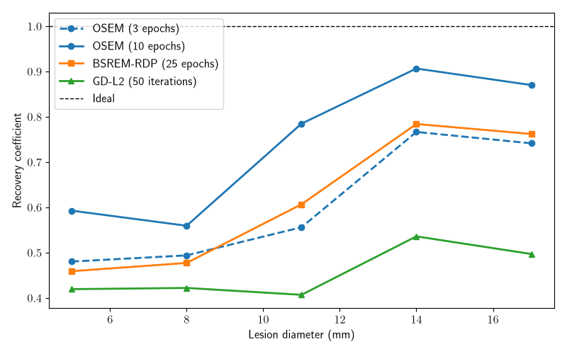
Recovery coefficients measure how much of the ground-truth activity within each lesion is recovered. For reconstruction \(\hat{x}\), ground truth \(x\), and lesion mask \(m\), the recovery coefficient is

\[\operatorname{RC}(\hat{x},x;m) = \frac{\sum_i \hat{x}_i m_i}{\sum_i x_i m_i + \varepsilon},\]

where \(\varepsilon\) is a small constant for numerical stability. A value of one indicates perfect activity recovery; in practice, small lesions are particularly difficult to recover at low counts.

recovery_coefficient = dinv.metric.RecoveryCoefficient()
rc_osem_early = []
rc_osem = []
rc_bsrem = []
rc_gd = []
for lesion_index in range(1, len(lesion_diameters) + 1):
    mask = lesion_mask == lesion_index
    rc_osem_early.append(recovery_coefficient(x_osem_early, x, mask=mask).item())
    rc_osem.append(recovery_coefficient(x_osem, x, mask=mask).item())
    rc_bsrem.append(recovery_coefficient(x_bsrem, x, mask=mask).item())
    rc_gd.append(recovery_coefficient(x_gd, x, mask=mask).item())

fig, axis = plt.subplots(figsize=(8, 5))
axis.plot(
    lesion_diameters,
    rc_osem_early,
    label=f"OSEM ({osem_early_iter} epochs)",
    color=method_colors["OSEM"],
    marker=method_markers["OSEM"],
    linestyle="--",
)
axis.plot(
    lesion_diameters,
    rc_osem,
    label=f"OSEM ({num_iter_osem} epochs)",
    color=method_colors["OSEM"],
    marker=method_markers["OSEM"],
)
axis.plot(
    lesion_diameters,
    rc_bsrem,
    label=f"BSREM-RDP ({num_epochs_bsrem} epochs)",
    color=method_colors["BSREM-RDP"],
    marker=method_markers["BSREM-RDP"],
)
axis.plot(
    lesion_diameters,
    rc_gd,
    label=f"GD-L2 ({num_iter_gd} iterations)",
    color=method_colors["GD-L2"],
    marker=method_markers["GD-L2"],
)
axis.axhline(1.0, color="black", linestyle="--", linewidth=1, label="Ideal")
axis.set_xlabel("Lesion diameter (mm)")
axis.set_ylabel("Recovery coefficient")
axis.legend()
fig.tight_layout()

References:

[1]

Johan Nuyts, Dirk Bequé, Patrick Dupont, and Luc Mortelmans. A concave prior penalizing relative differences for maximum-a-posteriori reconstruction in emission tomography. IEEE Transactions on Nuclear Science, 49(1):56–60, February 2002. doi:10.1109/TNS.2002.998681.

[2]

H.M. Hudson and R.S. Larkin. Accelerated image reconstruction using ordered subsets of projection data. IEEE Transactions on Medical Imaging, 13(4):601–609, December 1994. doi:10.1109/42.363108.

[3]

Lawrence A Shepp and Yehuda Vardi. Maximum likelihood reconstruction for emission tomography. IEEE Transactions on Medical Imaging, 1(2):113–122, 1982.

[4]

Sangtae Ahn and Jeffrey A. Fessler. Globally convergent image reconstruction for emission tomography using relaxed ordered subsets algorithms. IEEE Transactions on Medical Imaging, 22(5):613–626, May 2003. doi:10.1109/TMI.2003.812251.

🏷 Tags: Tomography, PET/SPECT