Blind Richardson-Lucy deconvolution

This example introduces the Richardson-Lucy algorithm for deconvolution in the blind setting, where both the underlying clean image and the blur kernel are unknown.

We first consider the non-blind problem

\[y = h * x,\]

where \(h\) is the known convolution kernel. Richardson-Lucy [1][2] is a deconvolution algorithm used when the data is corrupted by Poisson noise. Starting from a nonnegative image \(x^{(0)}\), it iterates

\[x^{(k+1)} = \frac{x^{(k)}}{h^\dagger * \mathbf{1}} \odot h^\dagger * \left(\frac{y}{h * x^{(k)}}\right),\]

where \(h^\dagger\) is the spatially flipped kernel, such that \(h^\dagger *\) is the adjoint of convolution by \(h\). All products and divisions outside convolutions are pointwise.

When \(h\) is unknown, blind Richardson-Lucy alternates these updates for the image \(x\) and the kernel \(h\). This is a classical, simple baseline for blind deconvolution. It can use regularization on the image and/or the kernel to improve performances.

Setup the physics

Here we consider a simple Gaussian blur kernel and a medium amount of Poisson noise.

import torch
import deepinv as dinv

torch.manual_seed(0)

device = dinv.utils.get_freer_gpu() if torch.cuda.is_available() else "cpu"
img_size = 128 if torch.cuda.is_available() else 64

psnr = dinv.metric.PSNR()
mae = dinv.metric.MAE()

gaussian_psf = dinv.physics.functional.gaussian_blur(
    psf_size=(17, 17),
    sigma=2.0,
    device=device,
)
kernel_init = torch.ones_like(gaussian_psf)
kernel_init = kernel_init / kernel_init.sum()
gain = 1 / 100

physics = dinv.physics.BlurFFT(
    img_size=(1, img_size, img_size),
    filter=gaussian_psf,
    device=device,
    noise_model=dinv.physics.PoissonNoise(
        gain=gain, normalize=True, clip_positive=True
    ),
)

Selected GPU 0 with 18053.4375 MiB free memory

Non-blind Richardson-Lucy on a grayscale image

In the non-blind setting, the kernel is known and the only unknown is the image. In deepinv, the non-blind Richardson-Lucy algorithm corresponds to the deepinv.optim.MLEM used on measurements involving a blur physics. It works both on grayscale and RGB images, but for simplicity we first consider grayscale images.

x_gray = dinv.utils.load_example(
    "SheppLogan.png",
    img_size=img_size,
    grayscale=True,
    resize_mode="resize",
    device=device,
)

y_gray = physics(x_gray)

data_fidelity = dinv.optim.PoissonLikelihood(gain=gain)
mlem = dinv.optim.MLEM(
    data_fidelity=data_fidelity,
    prior=None,
    max_iter=70 if torch.cuda.is_available() else 20,
    early_stop=True,
    thres_conv=1e-6,
    crit_conv="residual",
    verbose=True,
)

x_rl, metrics = mlem(
    y_gray,
    physics,
    x_gt=x_gray,
    compute_metrics=True,
)

dinv.utils.plot(
    {
        "Ground truth": x_gray,
        "Blurred": y_gray,
        "Richardson-Lucy": x_rl.clamp(0, 1),
    },
    subtitles=[
        "Reference",
        f"PSNR: {psnr(x_gray, y_gray).item():.2f} dB",
        f"PSNR: {psnr(x_gray, x_rl).item():.2f} dB",
    ],
    figsize=(9, 3),
    rescale_mode="clip",
    vmin=0,
    vmax=1,
)

dinv.utils.plot_curves(metrics)

• 
• 

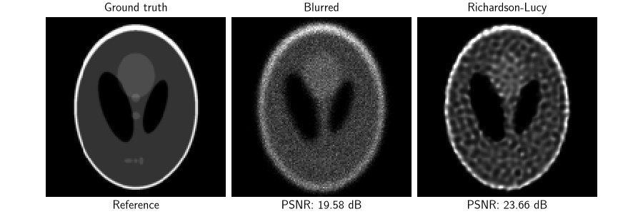
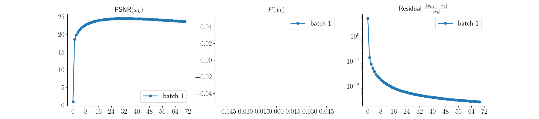
Blind Richardson-Lucy on clean data

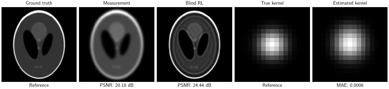
We now assume that both the clean image \(x\) and the blur kernel \(h\) are unknown. The convolution is written \(h * x\) when updating the image and \(x * h\) when updating the kernel. The blind Richardson-Lucy algorithm simply alternates the Richardson-Lucy updates for these two convolutions. The updates are given by:

\[h^{(k+1)} = \Pi_{\Delta}\left[\frac{h^{(k)}}{(x^{(k)})^\dagger * \mathbf{1}} \odot (x^{(k)})^\dagger * \left(\frac{y}{x^{(k)} * h^{(k)}}\right)\right],\]

and

\[x^{(k+1)} = \frac{x^{(k)}}{(h^{(k+1)})^\dagger * \mathbf{1}} \odot (h^{(k+1)})^\dagger * \left(\frac{y}{h^{(k+1)} * x^{(k)}}\right).\]

Here, \(z^\dagger\) denotes the spatially flipped \(z\), such that \(z^\dagger *\) is the adjoint of convolution by \(z\). The operation \(\Pi_{\Delta}\) keeps the kernel nonnegative and normalized to unit sum. The deepinv.optim.BlindRL class implements these alternating updates.

This algorithm is implemented under the deepinv.optim.BlindRL class. The number of iterations of each of the two updates can be controlled by the parameters x_steps and k_steps. Here, we set use_fft=True to compute the filter adjoint with FFTs.

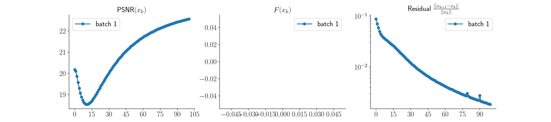
For simplicity we first test this algorithm on a clean measurement, i.e. without noise. In this case, the algorithm performs fairly well, with only some oscillation artefacts near the edges known as Gibbs phenomenon.

physics_clean = dinv.physics.Blur(
    filter=gaussian_psf,
    padding="circular",
    device=device,
)
y_clean = physics_clean(x_gray)

blindrl = dinv.optim.BlindRL(
    max_iter=100 if torch.cuda.is_available() else 40,
    init=(y_clean.clamp_min(1e-12), kernel_init),
    x_steps=1,
    k_steps=1,
    normalize_kernel=True,
    use_fft=True,
    verbose=True,
)
(x_blindrl, k_blindrl), metrics_clean_blind = blindrl(
    y_clean,
    x_gt=x_gray,
    compute_metrics=True,
)
x_blindrl = x_blindrl.clamp(0, 1)

dinv.utils.plot(
    {
        "Ground truth": x_gray,
        "Measurement": y_clean,
        "Blind RL": x_blindrl,
        "True kernel": gaussian_psf,
        "Estimated kernel": k_blindrl,
    },
    subtitles=[
        "Reference",
        f"PSNR: {psnr(x_gray, y_clean).item():.2f} dB",
        f"PSNR: {psnr(x_gray, x_blindrl).item():.2f} dB",
        "Reference",
        f"MAE: {mae(gaussian_psf, k_blindrl).item():.4f}",
    ],
    figsize=(13, 3),
    rescale_mode="clip",
    vmin=0,
    vmax=1,
)
dinv.utils.plot_curves(metrics_clean_blind)

• 
• 

Blind Richardson-Lucy on noisy data

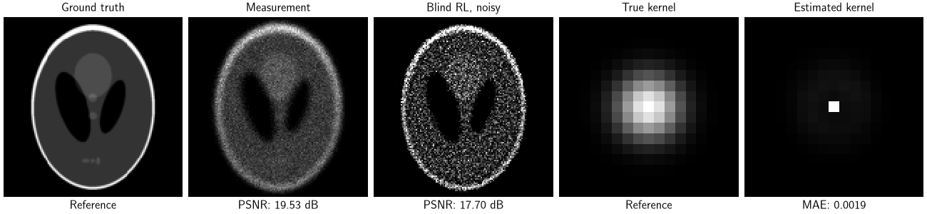
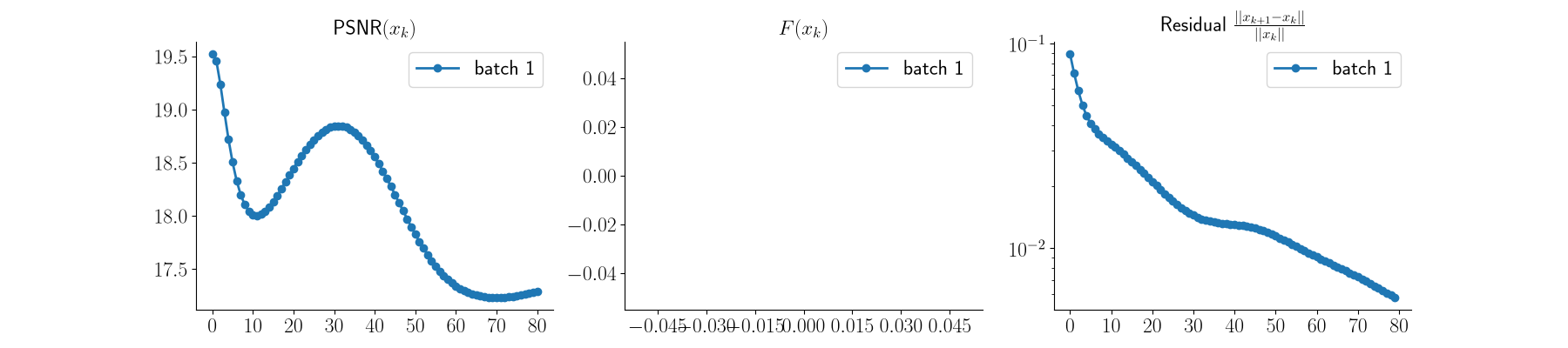
Blind Richardson-Lucy is much less stable when the data is noisy. Without regularization, the multiplicative updates tend to amplify noise and the blur kernel tends to converge very fast to a Dirac. The Dirac is unfortunately never a valid solution, because it corresponds to the situation where our input image \(y\) was already sharp.

Here we show an example with a medium amount of Poisson noise. The algorithm further degrades the image and is unable to recover the correct kernel.

y_noisy = physics(x_gray)

physics_clean.update_parameters(filter=gaussian_psf)
blindrl = dinv.optim.BlindRL(
    max_iter=80 if torch.cuda.is_available() else 40,
    init=(y_noisy.clamp_min(1e-12), kernel_init),
    x_steps=1,
    k_steps=1,
    normalize_kernel=True,
    use_fft=True,
    verbose=True,
)
(x_blindrl, k_blindrl), metrics = blindrl(
    y_noisy,
    x_gt=x_gray,
    compute_metrics=True,
)
x_blindrl = x_blindrl.clamp(0, 1)

dinv.utils.plot(
    {
        "Ground truth": x_gray,
        "Measurement": y_noisy,
        "Blind RL, noisy": x_blindrl,
        "True kernel": gaussian_psf,
        "Estimated kernel": k_blindrl,
    },
    subtitles=[
        "Reference",
        f"PSNR: {psnr(x_gray, y_noisy).item():.2f} dB",
        f"PSNR: {psnr(x_gray, x_blindrl).item():.2f} dB",
        "Reference",
        f"MAE: {mae(gaussian_psf, k_blindrl).item():.4f}",
    ],
    figsize=(13, 3),
    rescale_mode="clip",
    vmin=0,
    vmax=1,
)
dinv.utils.plot_curves(metrics)

• 
• 

One-Step-Late regularization

A standard heuristic to extend EM methods to the regularized setting is called One-Step-Late (OSL) regularization [3]. Since Richardson-Lucy is an instance of the EM algorithm, it can be extended to the regularized setting using OSL. For an image prior or regularizer \(R_x\) and a kernel regularizer \(R_h\), the denominators are modified using the current gradients:

\[h^{(k+1)} = \Pi_{\Delta}\left[\frac{h^{(k)}}{(x^{(k)})^\dagger * \mathbf{1} + \lambda_h \nabla R_h(h^{(k)})} \odot (x^{(k)})^\dagger * \left(\frac{y}{x^{(k)} * h^{(k)}}\right)\right].\]

\[x^{(k+1)} = \frac{x^{(k)}}{(h^{(k+1)})^\dagger * \mathbf{1} + \lambda_x \nabla R_x(x^{(k)})} \odot (h^{(k+1)})^\dagger * \left(\frac{y}{h^{(k+1)} * x^{(k)}}\right),\]

In the non-smooth case, the gradients are replaced by subgradients. This enables the use of any prior implementing the deepinv.optim.prior.Prior interface inside the deepinv.optim.BlindRL class. Remember that the OSL method is heuristic and in particular is not guaranteed to converge. Still it is fairly robust in most cases and computationally efficient compared to more sophisticated regularized algorithms. The image and kernel regularizers can be specified independently using the x_prior and k_prior arguments of the deepinv.optim.BlindRL class. 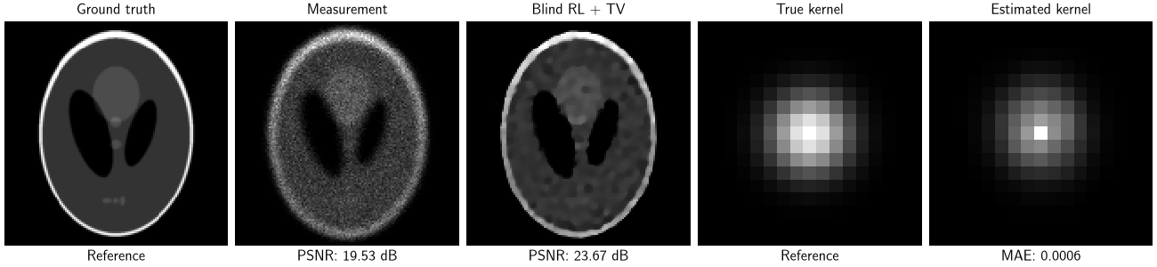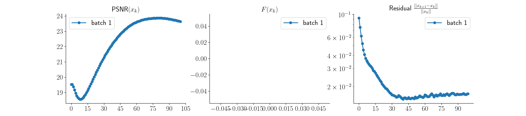Below, we use TV regularization on the image through the deepinv.optim.TVPrior class and no regularization on the kernel.

The image is a bit sharper and we get a better estimate of the kernel.

tv_prior = dinv.optim.TVPrior(n_it_max=10)

blindrl = dinv.optim.BlindRL(
    x_prior=tv_prior,
    k_prior=None,
    lambda_reg_x=0.015,
    lambda_reg_k=0.0,
    max_iter=100 if torch.cuda.is_available() else 40,
    init=(y_noisy.clamp_min(1e-12), kernel_init),
    x_steps=1,
    k_steps=1,
    normalize_kernel=True,
    use_fft=True,
    verbose=True,
)
(x_blindrl, k_blindrl), metrics = blindrl(
    y_noisy,
    x_gt=x_gray,
    compute_metrics=True,
)
x_blindrl = x_blindrl.clamp(0, 1)

dinv.utils.plot(
    {
        "Ground truth": x_gray,
        "Measurement": y_noisy,
        "Blind RL + TV": x_blindrl,
        "True kernel": gaussian_psf,
        "Estimated kernel": k_blindrl,
    },
    subtitles=[
        "Reference",
        f"PSNR: {psnr(x_gray, y_noisy).item():.2f} dB",
        f"PSNR: {psnr(x_gray, x_blindrl).item():.2f} dB",
        "Reference",
        f"MAE: {mae(gaussian_psf, k_blindrl).item():.4f}",
    ],
    figsize=(13, 3),
    rescale_mode="clip",
    vmin=0,
    vmax=1,
)
dinv.utils.plot_curves(metrics)

• 
• 

Blind Richardson-Lucy on an RGB image

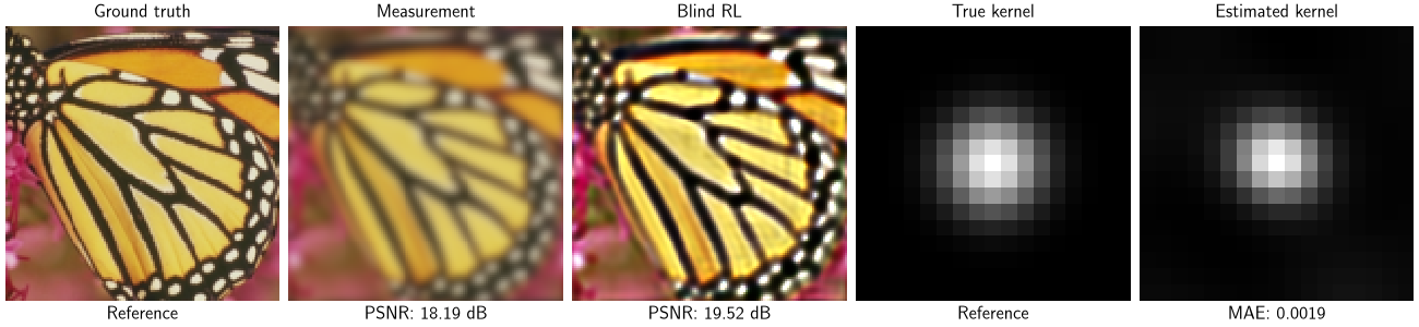
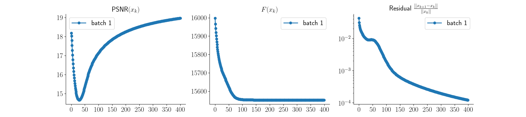
The same algorithm also works on RGB images. The blur kernel is shared across channels, and the kernel update aggregates information from all channels. Here we show a noiseless example, but in the noisy setting, regularization should again be used to avoid noise amplification and kernel collapse.

x_rgb = dinv.utils.load_example(
    "butterfly.png",
    img_size=img_size,
    grayscale=False,
    resize_mode="resize",
    device=device,
)

physics_clean.update_parameters(filter=gaussian_psf)
y_rgb = physics_clean(x_rgb)

blindrl = dinv.optim.BlindRL(
    max_iter=400 if torch.cuda.is_available() else 40,
    init=(y_rgb.clamp_min(1e-12), kernel_init),
    x_steps=1,
    k_steps=2,
    normalize_kernel=True,
    use_fft=True,
    verbose=True,
)
(x_blindrl, k_blindrl), metrics = blindrl(
    y_rgb,
    x_gt=x_rgb,
    compute_metrics=True,
)
x_blindrl = x_blindrl.clamp(0, 1)

dinv.utils.plot(
    {
        "Ground truth": x_rgb,
        "Measurement": y_rgb,
        "Blind RL": x_blindrl,
        "True kernel": gaussian_psf,
        "Estimated kernel": k_blindrl,
    },
    subtitles=[
        "Reference",
        f"PSNR: {psnr(x_rgb, y_rgb).item():.2f} dB",
        f"PSNR: {psnr(x_rgb, x_blindrl).item():.2f} dB",
        "Reference",
        f"MAE: {mae(gaussian_psf, k_blindrl).item():.4f}",
    ],
    figsize=(13, 3),
    rescale_mode="clip",
    vmin=0,
    vmax=1,
)
dinv.utils.plot_curves(metrics)

• 
• 

References:

[1]

William Hadley Richardson. Bayesian-based iterative method of image restoration. Journal of the Optical Society of America, 62(1):55, 1972. doi:10.1364/JOSA.62.000055.

[2]

L. B. Lucy. An iterative technique for the rectification of observed distributions. The Astronomical Journal, 79:745, 1974. doi:10.1086/111605.

[3]

Peter J. Green. On Use of the Em Algorithm for Penalized Likelihood Estimation. Journal of the Royal Statistical Society: Series B (Methodological), 52(3):443–452, 1990. doi:10.1111/j.2517-6161.1990.tb01798.x.