

WienerDeconvolution#
- class deepinv.models.WienerDeconvolution(lambda_reg=1.0, prior='laplacian', device='cpu')[source]#
Bases:
ReconstructorWiener deconvolution reconstruction model.
Solves the regularised least-squares problem
\[\hat{x} = \arg\min_x \; \frac{1}{2}\Vert Ax - y \Vert_2^2 + \frac{1}{2}\Vert \lambda^{1/2} \odot F x \Vert_2^2\]where \(F\) is the Fourier transform, \(\odot\) is element-wise multiplication, and \(\lambda\) is a per-frequency regularisation weight. The minimiser is available in closed form and is computed directly with FFTs, without an iterative solver.
The forward operator is a circular convolution, so \(A = F^{-1} \operatorname{diag}(H) F\) is diagonalised by \(F\). The minimiser is therefore given by the classical Wiener filter,
\[\hat{X}(f) = \frac{H^*(f)}{\vert H(f) \vert^2 + \lambda(f)} \, Y(f)\]in which \(\lambda(f)\) plays the role of a noise-to-signal PSD ratio \(S_n(f) / S_x(f)\): it is small where the signal dominates, and large where the measurement is mostly noise.
The arguments
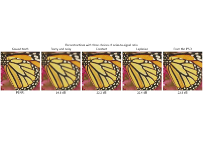
lambda_regandpriordefine \(\lambda\), specialising the problem into one of three cases.1. Flat Prior (
lambda_regis a scalar,prior="flat"orNone):\(\lambda(f) = \lambda\) is constant. Since \(F\) is unitary, the penalty reduces to standard Tikhonov regularisation:
\[\hat{x} = \arg\min_x \; \frac{1}{2}\Vert Ax - y \Vert_2^2 + \frac{\lambda}{2}\Vert x \Vert_2^2\]2. Laplacian Prior (
lambda_regis a scalar,prior="laplacian"):\(\lambda(f) = \lambda \left(|H_L(f)|^2 + \varepsilon\right)\), where \(H_L\) is the frequency response of the 2-D discrete Laplacian \(L\). Its power spectrum grows with frequency, so this penalises high frequencies more than low ones, enforcing spatial smoothness. By Parseval’s theorem this frequency-domain penalty is equivalent to a spatial penalty on \(Lx\), giving classical Wiener-Hunt deconvolution:
\[\hat{x} = \arg\min_x \; \frac{1}{2}\Vert Ax - y \Vert_2^2 + \frac{\lambda}{2}\left(\Vert L x \Vert_2^2 + \varepsilon \Vert x \Vert_2^2\right)\]where \(L\) is defined by the \(3 \times 3\) kernel:
\[\begin{split}L = \begin{bmatrix} 0 & -1 & 0 \\ -1 & 4 & -1 \\ 0 & -1 & 0 \end{bmatrix}\end{split}\]The \(\varepsilon\) term is numerically negligible (\(\varepsilon = 10^{-9}\)), but it keeps the DC component regularised: the Laplacian has \(|H_L(0)|^2 = 0\), so without it the mean of the image would be left entirely unregularised.
3. Custom Tensor (
lambda_regis a user-provided tensor):\(\lambda(f)\) is taken directly from the tensor, and
prioris ignored. This is the case to use when the noise and signal PSDs are known or have been estimated.Note
Only
BlurFFTis supported, since Wiener deconvolution requires a circular convolution.Denoisingcannot express frequency-domain regularisation at all (see the tip below);MRIcould, but subsamples the spectrum rather than blurring it, so the result would not be a deconvolution.Tip
Denoising is the special case of deconvolution in which the filter is a unit impulse. It is not supported through
Denoising, whose SVD basis is the identity rather than the Fourier basis, and which therefore cannot express any frequency-domain prior. Instead, build aBlurFFTwith a filter that is zero except for a1at its centre:impulse = torch.zeros(1, 1, 3, 3) impulse[0, 0, 1, 1] = 1.0 physics = BlurFFT(img_size=(C, H, W), filter=impulse)
This gives \(A = I\) together with a Fourier SVD basis, so
prior="laplacian"and a frequency-dependent tensorlambda_regboth apply. Effective Wiener smoothing requires such a frequency-dependent weighting: a scalar \(\lambda\) shrinks all frequencies uniformly.- Parameters:
lambda_reg (float, torch.Tensor) –
Regularisation parameter \(\lambda\) controlling the trade-off between data fidelity and regularisation. Larger values produce smoother (more regularised) reconstructions.
If a scalar
float, it is combined withprior(as detailed above). Settinglambda_reg=0returns the pseudo-inverse (no regularisation). A 0-dim tensor holds a single value and is treated the same way.If a
torch.Tensorwith one or more dimensions, it is a frequency-dependent NSR (noise-to-signal PSD ratio, \(\lambda(f) = S_n(f) / S_x(f)\)), andprioris ignored. It must be 4-D, of shape(B, C, H, W // 2 + 1), the half spectrum returned bytorch.fft.rfft2();BandCmay be1to broadcast. Entries equal to zero are clamped to a small positive value to avoid a division by zero.
prior (str, None) –
Regularisation prior. Only used when
lambda_regis a scalar. Default:"laplacian"."laplacian": Uses the power spectrum of the 2-D discrete Laplacian to build a frequency-varying regularisation, penalising high frequencies more than low frequencies (Wiener-Hunt model).Noneor"flat": Flat (constant) regularisation.
device (str, torch.device) – Device for the model. Default:
"cpu".
- Examples:
Wiener deconvolution of a blurred image with a flat prior:
>>> import torch
>>> from deepinv.physics import BlurFFT
>>> from deepinv.models import WienerDeconvolution
>>> x = torch.randn(1, 1, 8, 8)
>>> filter = torch.ones(1, 1, 3, 3) / 9.0
>>> physics = BlurFFT(img_size=(1, 8, 8), filter=filter)
>>> model = WienerDeconvolution(lambda_reg=1.0)
>>> with torch.no_grad():
...     x_hat = model(physics(x), physics)
>>> x_hat.shape
torch.Size([1, 1, 8, 8])
- forward(y, physics, **kwargs)[source]#
Reconstruct an image from measurements using Wiener deconvolution.
- Parameters:
y (torch.Tensor) – Measurement tensor.
physics (deepinv.physics.Physics) – Forward physics operator. Must be an instance of
BlurFFT. For denoising, use aBlurFFTbuilt with a unit-impulse filter (see the class docstring).kwargs – Accepted for compatibility with the
Reconstructorinterface and ignored. The reconstruction is fully determined bylambda_regandprior, which are set on the model at construction; passing them here has no effect.
- Returns:
Reconstructed image tensor.
- Return type:
- Raises:
ValueError – If
physicsis not aBlurFFT, or ifprioris not one of(None, "flat", "laplacian").
Examples using WienerDeconvolution:#
Wiener deconvolution with frequency-dependent regularization