Wiener deconvolution with frequency-dependent regularization

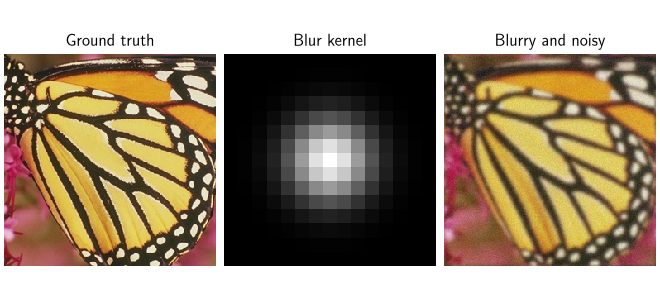
Deblurring is the inverse problem of recovering an image \(x\) from a blurred measurement. This example uses the forward model \(y = \forw{x} + \epsilon\), where \(A\) is a convolution and \(\epsilon\) is additive noise. Wiener deconvolution [1] is a classical learning-free solution. When \(A\) is a circular convolution it is diagonalized by the Fourier transform, so the regularized least-squares solution is available in closed form,

\[\hat{X}(f) = \frac{H^*(f)}{\lvert H(f) \rvert^2 + \lambda(f)} \, Y(f)\]

where \(\hat{X}\) and \(Y\) are the Fourier transforms of the reconstruction and the measurement, \(H\) is the transfer function of the blur, and \(\lambda\) acts as a noise-to-signal power ratio \(S_n(f) / S_x(f)\). The ratio is small where the signal dominates and large where the measurement is mostly noise.

The regularization acts in the Fourier domain, so \(\lambda\) can take a different value at each frequency. This example compares the three ways of specifying \(\lambda\) in deepinv.models.WienerDeconvolution: a constant, a Laplacian prior, and a ratio computed from the power spectra of the signal and the noise. It closes with the special case of denoising, where \(A\) is the identity and a constant \(\lambda\) can only rescale the image.

import torch
import deepinv as dinv

# For reproducibility
torch.manual_seed(0)

# Select the device
device = dinv.utils.get_device()

# Load in the test image
x = dinv.utils.load_example("butterfly.png", img_size=256).to(device)

# Define the forward model: BlurFFT applies the Gaussian kernel as a circular
# convolution, and the noise model adds white Gaussian noise to the measurement
sigma_noise = 0.03
kernel = dinv.physics.functional.gaussian_blur(sigma=(2, 2), device=device)
physics = dinv.physics.BlurFFT(
    img_size=x.shape[1:],
    filter=kernel,
    noise_model=dinv.physics.GaussianNoise(sigma=sigma_noise),
    device=device,
)

# Compute the blurry, noisy measurement
y = physics(x)

# Define the metric
psnr_fn = dinv.metric.PSNR()

# Display the image, the blur kernel and the measurement
dinv.utils.plot(
    [x, kernel, y],
    ["Ground truth", "Blur kernel", "Blurry and noisy"],
    figsize=(6.6, 3.0),
)

Selected GPU 0 with 20138.4375 MiB free memory

Why regularization is needed

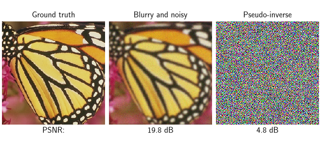
The circular convolution is diagonalized by the Fourier transform, so the unregularized least-squares solution, or pseudo-inverse, divides the spectrum of the measurement by the transfer function,

\[\hat{X}(f) = \frac{Y(f)}{H(f)}\]

With \(Y = H X + N\), where \(N\) is the noise spectrum, this gives \(\hat{X} = X + N / H\): the blur is inverted exactly, and only the noise is amplified, wherever \(H(f)\) is small. Blur kernels typically attenuate high frequencies, and for the Gaussian kernel used here \(H(f)\) decays rapidly, so the result of the inversion is dominated by amplified noise.

# Compute the pseudo-inverse
x_pinv = physics.A_dagger(y).clip(0, 1)

# Plot the pseudo-inverse alongside the measurement
dinv.utils.plot(
    [x, y, x_pinv],
    ["Ground truth", "Blurry and noisy", "Pseudo-inverse"],
    subtitles=[
        "PSNR:",
        f"{psnr_fn(y, x).item():.1f} dB",
        f"{psnr_fn(x_pinv, x).item():.1f} dB",
    ],
    rescale_mode="clip",
    figsize=(6.6, 3.0),
)

A constant noise-to-signal ratio

The simplest choice for \(\lambda\) is a constant, which corresponds to assuming the noise-to-signal ratio is the same at every frequency. Since the Fourier transform is unitary, a constant weight in frequency is the same weight in space, and the penalty becomes \(\lambda \lVert x \rVert^2 / 2\). This is Tikhonov regularization, obtained with prior=None.

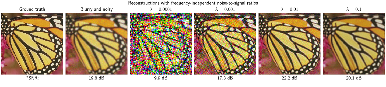
The value of \(\lambda\) controls the trade-off between noise amplification and over-smoothing. Small values leave the reconstruction close to the pseudo-inverse and retain its amplified noise; large values attenuate the high frequencies that carry image detail.

# Values of lambda to compare
lambdas = [1e-4, 1e-3, 1e-2, 1e-1]

# Reconstruct with each value
x_flat = []
for lambda_reg in lambdas:
    model = dinv.models.WienerDeconvolution(lambda_reg=lambda_reg, prior=None)
    x_flat.append(model(y, physics).clip(0, 1))

# Compute the performance metrics
psnr_flat = [psnr_fn(x_hat, x).item() for x_hat in x_flat]

# Plot the reconstruction for each value
dinv.utils.plot(
    [x, y] + x_flat,
    ["Ground truth", "Blurry and noisy"]
    + [rf"$\lambda = {lambda_reg:g}$" for lambda_reg in lambdas],
    subtitles=["PSNR:", f"{psnr_fn(y, x).item():.1f} dB"]
    + [f"{p:.1f} dB" for p in psnr_flat],
    suptitle="Reconstructions with frequency-independent noise-to-signal ratios",
    rescale_mode="clip",
    figsize=(13.2, 3.0),
)

# Keep the best value for the comparisons below
best_lambda = lambdas[int(torch.tensor(psnr_flat).argmax())]
print(f"Best constant lambda: {best_lambda:g} ({max(psnr_flat):.2f} dB)")

/local/pberna03/actions-runner/_work/deepinv/deepinv/deepinv/utils/plotting.py:519: UserWarning: This figure was using a layout engine that is incompatible with subplots_adjust and/or tight_layout; not calling subplots_adjust.
  fig.subplots_adjust(top=0.75)
Best constant lambda: 0.01 (22.21 dB)

A Laplacian prior

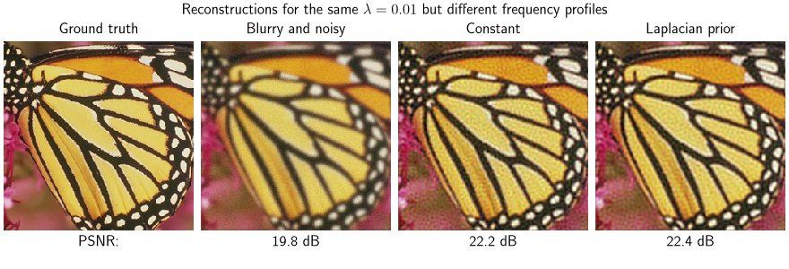
Natural images have most of their energy at low frequencies, while white noise is spread evenly across them, so the ideal ratio \(S_n / S_x\) is small at low frequencies and large at high ones. No constant can match a ratio that varies with frequency: a compromise value over-regularizes where the signal dominates and under-regularizes where the noise does. Setting prior="laplacian" replaces the constant by

\[\lambda(f) = \lambda \left( \lvert H_L(f) \rvert^2 + \varepsilon \right)\]

where \(H_L\) is the transfer function of a discrete Laplacian filter. The constant \(\varepsilon\) is added because \(\lvert H_L(f) \rvert^2\) vanishes at zero frequency. By Parseval’s theorem the penalty is then \(\lambda ( \lVert L x \rVert^2 + \varepsilon \lVert x \rVert^2 ) / 2\), which penalizes high frequencies more strongly than low ones. This is the default.

# Reconstruct with the Laplacian prior at the best constant lambda
model = dinv.models.WienerDeconvolution(lambda_reg=best_lambda, prior="laplacian")
x_laplacian = model(y, physics).clip(0, 1)

# Plot the reconstructions from the constant and the Laplacian prior
dinv.utils.plot(
    [x, y, x_flat[lambdas.index(best_lambda)], x_laplacian],
    ["Ground truth", "Blurry and noisy", "Constant", "Laplacian prior"],
    subtitles=[
        "PSNR:",
        f"{psnr_fn(y, x).item():.1f} dB",
        f"{psnr_flat[lambdas.index(best_lambda)]:.1f} dB",
        f"{psnr_fn(x_laplacian, x).item():.1f} dB",
    ],
    suptitle=rf"Reconstructions for the same $\lambda = {best_lambda:g}$ "
    "but different frequency profiles",
    rescale_mode="clip",
    figsize=(8.8, 3.0),
)

/local/pberna03/actions-runner/_work/deepinv/deepinv/deepinv/utils/plotting.py:519: UserWarning: This figure was using a layout engine that is incompatible with subplots_adjust and/or tight_layout; not calling subplots_adjust.
  fig.subplots_adjust(top=0.75)

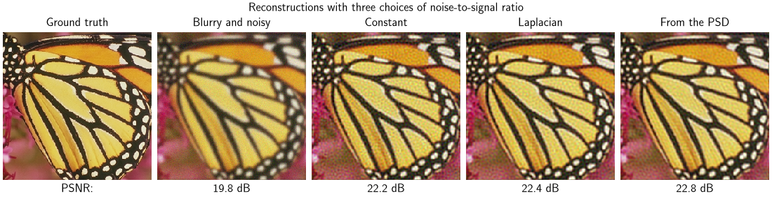
A ratio computed from the power spectra

A tensor passed as lambda_reg specifies \(\lambda(f)\) directly, allowing an arbitrary dependence on frequency that neither a constant nor the Laplacian prior can represent. Setting the tensor to the ratio of the noise and signal power spectra,

\[\lambda(f) = \frac{S_n(f)}{S_x(f)}\]

recovers the filter derived by Wiener. Every reconstruction in this example is a linear estimator: the measurement spectrum is multiplied by a fixed function of frequency, so the reconstruction depends linearly on \(y\). Among all such estimators, this choice of \(\lambda\) minimizes the expected squared error when \(S_x\) and \(S_n\) are the true power spectra. The noise is white, so \(S_n(f) = \sigma^2\) is constant across frequencies.

The tensor is broadcast against the half spectrum produced by the real FFT, of shape (B, C, H, W // 2 + 1), so a single spectrum shared by the colour channels is supplied as (1, 1, H, W // 2 + 1). Here \(S_x\) is estimated from the ground-truth image, which is not available in practice. The PSNR below is therefore optimistic: it shows what a frequency-dependent ratio achieves when the signal spectrum is known exactly. In an application \(S_x\) would be estimated from similar images, or assumed to follow a parametric model.

# Power spectral density of the signal, averaged into a single spectrum shared by
# the colour channels.  Averaging reduces the variance of the estimate, as would
# averaging over a set of similar images in practice
signal_psd = (torch.fft.rfft2(x, norm="ortho").abs() ** 2).mean(1, keepdim=True)

# Noise-to-signal ratio, for white noise of variance sigma^2.  The clamps keep it
# finite at frequencies where the signal spectrum is close to zero
nsr = (sigma_noise**2 / signal_psd.clamp(min=1e-12)).clamp(max=1e6)

# Reconstruct with the per-frequency ratio
model = dinv.models.WienerDeconvolution(lambda_reg=nsr)
x_psd = model(y, physics).clip(0, 1)

# Plot the reconstructions from the three choices of lambda
dinv.utils.plot(
    [x, y, x_flat[lambdas.index(best_lambda)], x_laplacian, x_psd],
    ["Ground truth", "Blurry and noisy", "Constant", "Laplacian", "From the PSD"],
    subtitles=[
        "PSNR:",
        f"{psnr_fn(y, x).item():.1f} dB",
        f"{psnr_flat[lambdas.index(best_lambda)]:.1f} dB",
        f"{psnr_fn(x_laplacian, x).item():.1f} dB",
        f"{psnr_fn(x_psd, x).item():.1f} dB",
    ],
    suptitle="Reconstructions with three choices of noise-to-signal ratio",
    rescale_mode="clip",
    figsize=(11.0, 3.0),
)

/local/pberna03/actions-runner/_work/deepinv/deepinv/deepinv/utils/plotting.py:519: UserWarning: This figure was using a layout engine that is incompatible with subplots_adjust and/or tight_layout; not calling subplots_adjust.
  fig.subplots_adjust(top=0.75)

Special case: denoising

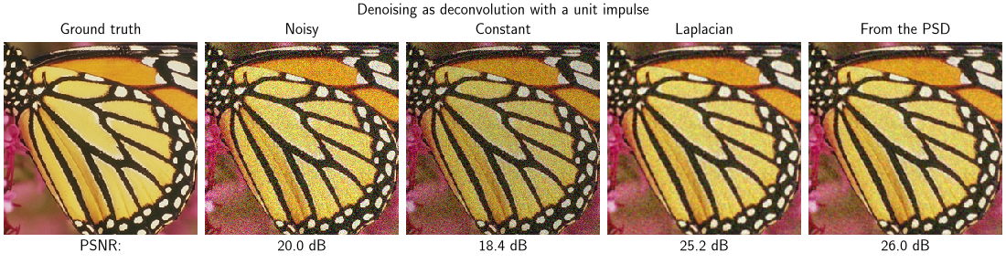
Wiener filtering applies to denoising as well as deblurring. Denoising is the case where the forward operator is the identity, obtained here by taking the blur kernel to be a unit impulse. Any circular convolution is diagonalized by the Fourier transform, so the frequency-dependent priors above apply here too. With \(H(f) = 1\) at every frequency, the Wiener filter reduces to

\[\hat{X}(f) = \frac{Y(f)}{1 + \lambda(f)}\]

which is a per-frequency shrinkage of the measurement, with no deconvolution.

This makes the role of the frequency profile explicit. A constant \(\lambda\) reduces the expression further to \(Y(f) / (1 + \lambda)\), the same factor at every frequency. Signal and noise are rescaled alike, so the signal-to-noise ratio is unchanged whatever the value of \(\lambda\). Only a \(\lambda\) that varies with frequency can denoise.

# Noise level and regularization strength used in this section
sigma_denoising = 0.1
lambda_denoising = 0.2

# Express denoising as a convolution with a unit impulse
impulse = torch.zeros(1, 1, 3, 3, device=device)
impulse[0, 0, 1, 1] = 1.0
physics_denoising = dinv.physics.BlurFFT(
    img_size=x.shape[1:],
    filter=impulse,
    noise_model=dinv.physics.GaussianNoise(sigma=sigma_denoising),
    device=device,
)

# Compute the noisy measurement
y_noisy = physics_denoising(x)

# Noise-to-signal ratio at this noise level, reusing the signal spectrum above
nsr_denoising = (sigma_denoising**2 / signal_psd.clamp(min=1e-12)).clamp(max=1e6)

# Reconstruct with the same three choices of lambda as above, the constant and
# the Laplacian prior sharing a single value
x_dn_flat = dinv.models.WienerDeconvolution(lambda_reg=lambda_denoising, prior=None)(
    y_noisy, physics_denoising
).clip(0, 1)
x_dn_laplacian = dinv.models.WienerDeconvolution(
    lambda_reg=lambda_denoising, prior="laplacian"
)(y_noisy, physics_denoising).clip(0, 1)
x_dn_psd = dinv.models.WienerDeconvolution(lambda_reg=nsr_denoising)(
    y_noisy, physics_denoising
).clip(0, 1)

# Plot the noisy image and the three denoised reconstructions
dinv.utils.plot(
    [x, y_noisy, x_dn_flat, x_dn_laplacian, x_dn_psd],
    ["Ground truth", "Noisy", "Constant", "Laplacian", "From the PSD"],
    subtitles=[
        "PSNR:",
        f"{psnr_fn(y_noisy, x).item():.1f} dB",
        f"{psnr_fn(x_dn_flat, x).item():.1f} dB",
        f"{psnr_fn(x_dn_laplacian, x).item():.1f} dB",
        f"{psnr_fn(x_dn_psd, x).item():.1f} dB",
    ],
    suptitle="Denoising as deconvolution with a unit impulse",
    rescale_mode="clip",
    figsize=(11.0, 3.0),
)

/local/pberna03/actions-runner/_work/deepinv/deepinv/deepinv/utils/plotting.py:519: UserWarning: This figure was using a layout engine that is incompatible with subplots_adjust and/or tight_layout; not calling subplots_adjust.
  fig.subplots_adjust(top=0.75)

The Laplacian profile attenuates high frequencies, trading resolution for noise reduction. As in the deblurring case, the ratio from the PSD is computed from the ground-truth spectrum, so its margin over the Laplacian profile is optimistic. Because the filter is linear and shift-invariant, it applies the same frequency response everywhere in the image, so unlike the learned denoisers in the library it cannot smooth flat regions while preserving edges. Wiener denoising is useful as a baseline and as a fast initialization for iterative methods; see Benchmarking pretrained denoisers for a benchmark of the pretrained denoisers.

See deepinv.models.WienerDeconvolution and the user guide for details.

References:

[1]

Norbert Wiener. Extrapolation, Interpolation, and Smoothing of Stationary Time Series: With Engineering Applications. MIT Press, Cambridge, MA, 1949.