Motion simulation and motion-compensated reconstruction

Many imaging modalities are not acquired all at once but sequentially in “shots”, e.g. kspace lines in MRI or projections in CT. Since the time between shots is non-negligible, the subject may move during scanning, and reconstructions that assume a static subject will be motion-corrupted. Modelling a transform per shot allows us to simulate this motion corruption and, given the motion parameters, to compensate for it during reconstruction.

Here we focus on Cartesian MRI, where kspace lines are sampled sequentially. We model the motion corruption by modelling sequential acquisition with deepinv.physics.SequentialMultiCoilMRI, by using a transform that applies a transformation per time-step. If we ignore the motion during reconstruction, this gives motion-corrupted/blind reconstructions. However, if we are able to model the motion transformation parameters during reconstruction, we can compensate/correct for the motion.

We show rigid motion (deepinv.transform.projective.Euclidean) using a linear rotation trajectory and a random Brownian rotation + translation trajectory, and a non-rigid deformation (deepinv.transform.CPABDiffeomorphism) using a periodic trajectory.

See Dynamic & time-resolved imaging for further details on how to use transform and transform_params for modelling sequential/”time-resolved” physics.

Note

In this example we simulate acquisition by simulating coil maps, mask and motion trajectory. In practice these are estimated from the data, i.e. the mask is known from the acquisition, the coil maps from deepinv.physics.MultiCoilMRI.estimate_coil_maps(), and the motion trajectory from motion estimation (not covered here).

import matplotlib.pyplot as plt
import torch
import deepinv as dinv

device = dinv.utils.get_device()
torch.manual_seed(0)
rng = torch.Generator(device=device).manual_seed(1)

import matplotlib as mpl

mpl.rcParams["animation.html"] = "jshtml"

Selected GPU 0 with 24509.3125 MiB free memory

Load a brain image

We use a sample ground truth image from FastMRI and simulate a fully-sampled mask and simulate coil maps. The mask is sequential: e.g. time-step contains non-overlapping kspace samples.

dataset = dinv.datasets.SimpleFastMRISliceDataset(
    "data", anatomy="brain", download=True, use_dict_output=True
)
x = dataset[0]["x"].unsqueeze(0).to(device)  # (1, 2, H, W)

n_frames = 32

mask_generator = dinv.physics.generator.SequentialMaskGenerator(
    dinv.physics.generator.RandomMaskGenerator(
        (2, *x.shape[-2:]), acceleration=1, device=device
    ),
    T=n_frames,
)
mask = mask_generator.step()["mask"]

  0%|          | 0/820534 [00:00<?, ?it/s]
100%|██████████| 801k/801k [00:00<00:00, 13.4MB/s]

Simulate linear rotation motion-corruption

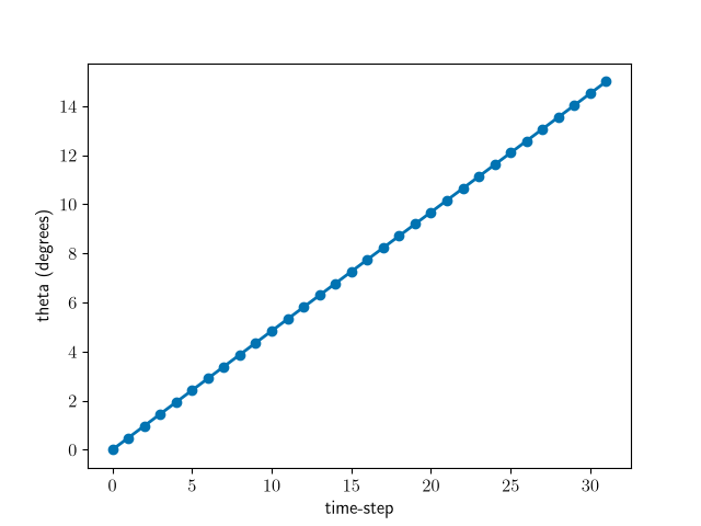
We rotate the object by theta degrees at each time-step, simulating a linear trajectory. The transform param trajectory is of shape B,T,... where the T dim matches the timesteps of the physics.

theta = torch.linspace(0, 15, n_frames, device=device).unsqueeze(0)

plt.figure()
plt.plot(theta.squeeze().cpu())
plt.ylabel("theta (degrees)")
plt.xlabel("time-step")
plt.show()

Construct motion physics by assuming knowledge of the transform params.

Note

The 1st axis of transform params is typically n_trans for multiple transforms per image for data augmentation or equivariance. However, here we set index_params_into_batch=True so that each image in the batch follows its own trajectory, i.e. params of shape (B,T).

transform = dinv.transform.projective.Euclidean(
    index_params_into_batch=True, padding="zeros"
)

physics = dinv.physics.SequentialMultiCoilMRI(
    img_size=x.shape[1:],
    mask=mask,
    coil_maps=4,  # simulated
    transform=transform,
    transform_params={"theta_z": theta},
    device=device,
)

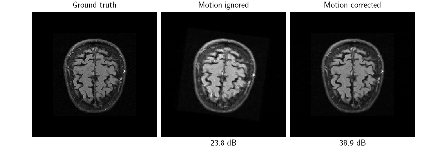
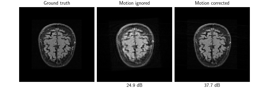
Simulate measurements, then show blind reconstruction vs. motion-corrected reconstruction. The motion-blind adjoint smears the anatomy whereas the motion-compensated adjoint rotates each frame back before summing over time.

y = physics(x)
x_blind = physics.A_adjoint(y, blind=True)
x_aware = physics.A_adjoint(y)

metric = dinv.metric.PSNR(complex_abs=True)

dinv.utils.plot(
    {
        "Ground truth": x,
        f"Motion ignored": x_blind,
        f"Motion corrected": x_aware,
    },
    subtitles=[
        "",
        f"{metric(x_blind, x).item():.1f} dB",
        f"{metric(x_aware, x, x).item():.1f} dB",
    ],
    figsize=(9, 3),
)

Tip

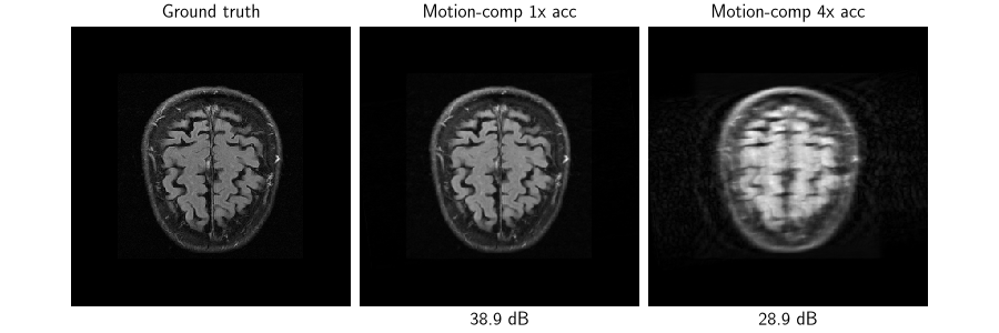
Even though acceleration=1, the motion means that kspace of the static object is not fully sampled (PSNR < 80dB), as each time-step only samples its own kspace lines of the moved object. Therefore the problem is not perfectly invertible and the motion-corrected adjoint is not perfect even when the motion is perfectly modelled, motivating the use of more advanced reconstruction methods.

The problem becomes even harder with accelerated MRI, i.e. acceleration>1. Below we simulate a 4x accelerated mask:

accelerated_generator = dinv.physics.generator.SequentialMaskGenerator(
    dinv.physics.generator.RandomMaskGenerator(
        (2, *x.shape[-2:]), acceleration=4, device=device
    ),
    T=n_frames,
)

physics.update(**accelerated_generator.step())
y_4x = physics(x)
x_4x_aware = physics.A_adjoint(y_4x)


dinv.utils.plot(
    {
        "Ground truth": x,
        f"Motion-comp 1x acc": x_aware,
        f"Motion-comp 4x acc": x_4x_aware,
    },
    subtitles=[
        "",
        f"{metric(x_aware, x).item():.1f} dB",
        f"{metric(x_4x_aware, x).item():.1f} dB",
    ],
    figsize=(9, 3),
)

physics.update(mask=mask)  # revert

Simulate Euclidean motion with a Brownian trajectory

We now combine the rotation with random translations giving Euclidean transformations. We model a random Brownian trajectory for the parameters (rotation angle and shifts)

physics_generator = (
    dinv.physics.generator.BrownianGenerator(
        "theta_z", T=n_frames, sigma=6.0, bound=15.0, device=device, rng=rng
    )
    + dinv.physics.generator.BrownianGenerator(
        "shift_x", T=n_frames, sigma=4.0, bound=10.0, device=device, rng=rng
    )
    + dinv.physics.generator.BrownianGenerator(
        "shift_y", T=n_frames, sigma=4.0, bound=10.0, device=device, rng=rng
    )
)

params = physics_generator.step()

plt.figure()
for label, values in params.items():
    plt.plot(values[0].cpu(), label=label)
plt.legend()
plt.xlabel("time-step")
plt.show()

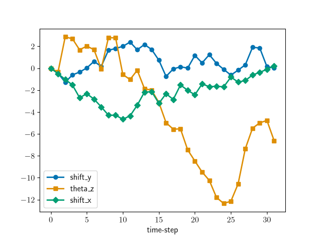
Update the physics with the new transform params:

physics.update(**params)

The moving object (left) and the cumulative k-space coverage (right) over the acquisition:

anim = dinv.utils.plot_videos(
    [
        torch.stack(
            [
                physics.transform.transform(
                    x, **{k: p[:, t] for k, p in params.items()}
                )
                for t in range(n_frames)
            ],
            dim=2,
        ),
        mask.cumsum(dim=2).clamp(max=1),
    ],
    titles=["Moving object", "k-space coverage"],
    return_anim=True,
)
anim

Once Loop Reflect

Simulate measurements, then show blind reconstruction vs. motion-corrected reconstruction:

y = physics(x)
x_blind = physics.A_adjoint(y, blind=True)
x_aware = physics.A_adjoint(y)

dinv.utils.plot(
    {
        "Ground truth": x,
        f"Motion ignored": x_blind,
        f"Motion corrected": x_aware,
    },
    subtitles=[
        "",
        f"{metric(x_blind, x).item():.1f} dB",
        f"{metric(x_aware, x, x).item():.1f} dB",
    ],
    figsize=(9, 3),
)

Non-rigid motion on a cardiac scan

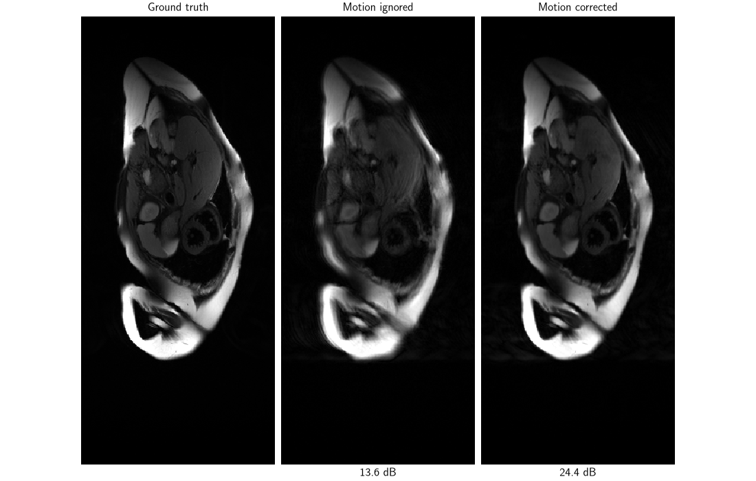
The heartbeat deforms the anatomy non-rigidly and periodically. We simulate this with a diffeomorphism whose parameters follow a fixed direction scaled by a sinusoidal trajectory. The ground truth is a T2-weighted, fully-sampled cardiac scan (iFFT + virtual coil combination).

x = dinv.utils.demo.load_example("demo_cmrxrecon2025_T2w_vcc.pt").to(device)

transform = dinv.transform.CPABDiffeomorphism(
    index_params_into_batch=True, n_trans=1, device=device
)

Simulate periodic motion of the diffeomorphism params by defining your own simple trajectory generator, combined with the mask generator from before, generating masks of the new image size:

class SinusoidTrajectoryGenerator(dinv.physics.generator.TrajectoryGenerator):
    def __init__(self, param_key, T, direction, n_periods, **kwargs):
        super().__init__(param_key, T, **kwargs)
        self.direction = direction
        self.n_periods = n_periods

    def sample_trajectory(self, batch_size):
        phase = torch.linspace(
            0, 2 * torch.pi * self.n_periods, self.T, **self.factory_kwargs
        )
        return (self.direction * phase.sin()[:, None]).expand(batch_size, -1, -1)


physics_generator = (
    SinusoidTrajectoryGenerator(
        "diffeo",
        T=n_frames,
        direction=torch.tensor(
            [0.3, -0.2, 0.2, 0.0, -0.3, 0.4, -0.4, 0.1], device=device
        ),
        n_periods=2,  # two heartbeats
        device=device,
    )
    + mask_generator
)

params = physics_generator.step(img_size=x.shape[-2:])
param, mask = params["diffeo"], params["mask"]

plt.figure()
for i in range(param.shape[-1]):
    plt.plot(param[0, :, i].cpu(), label=f"Diffeo param {i}")
plt.legend()
plt.xlabel("time-step")
plt.show()

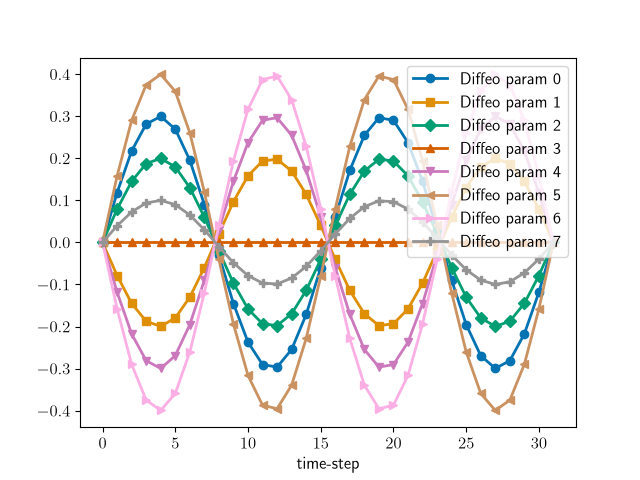
Construct motion physics with the new transform and update it with the params like before:

physics = dinv.physics.SequentialMultiCoilMRI(
    img_size=x.shape[1:], coil_maps=4, transform=transform, device=device
)
physics.update(**params)

The moving object (left) and the cumulative k-space coverage (right) over the acquisition:

anim = dinv.utils.plot_videos(
    [
        torch.stack(
            [transform.transform(x, diffeo=param[:, t]) for t in range(n_frames)], dim=2
        ),
        mask.cumsum(dim=2).clamp(max=1),
    ],
    titles=["Moving object", "k-space coverage"],
    return_anim=True,
    rescale_mode="clip",
    vmax=x.max() / 2,
    figsize=(7, 7),
)
anim

Once Loop Reflect

Simulate measurements, then show blind reconstruction vs. motion-corrected reconstruction:

y = physics(x)
x_blind = physics.A_adjoint(y, blind=True)
x_aware = physics.A_adjoint(y)

dinv.utils.plot(
    {
        "Ground truth": x,
        f"Motion ignored": x_blind,
        f"Motion corrected": x_aware,
    },
    subtitles=[
        "",
        f"{metric(x_blind, x).item():.1f} dB",
        f"{metric(x_aware, x, x).item():.1f} dB",
    ],
    figsize=(11, 7),
    rescale_mode="clip",
    vmax=x.max() / 2,
)